2016:Discovery of Repeated Themes & Sections Results/
THESE AREN'T THE 2016 RESULTS YET. THE PAGE IS UNDER CONSTRUCTION.
Contents
Introduction
The task: algorithms take a piece of music as input, and output a list of patterns repeated within that piece. A pattern is defined as a set of ontime-pitch pairs that occurs at least twice (i.e., is repeated at least once) in a piece of music. The second, third, etc. occurrences of the pattern will likely be shifted in time and/or transposed, relative to the first occurrence. Ideally an algorithm will be able to discover all exact and inexact occurrences of a pattern within a piece, so in evaluating this task we are interested in both:
- (1) to what extent an algorithm can discover one occurrence, up to time shift and transposition, and;
- (2) to what extent it can find all occurrences.
The metrics establishment recall, establishment precision and establishment F1 address (1), and the metrics occurrence recall, occurrence precision, and occurrence F1 address (2).
Contribution
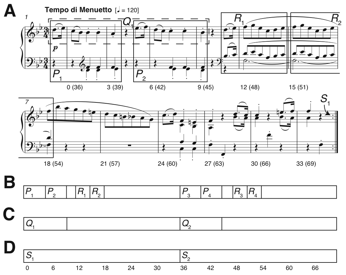
Existing approaches to music structure analysis in MIR tend to focus on segmentation (e.g., Weiss & Bello, 2010). The contribution of this task is to afford access to the note content itself (please see the example in Fig. 1A), requiring algorithms to do more than label time windows (e.g., the segmentations in Figs. 1B-D). For instance, a discovery algorithm applied to the piece in Fig. 1A should return a pattern corresponding to the note content of and , as well as a pattern corresponding to the note content of . This is because occurs again independently of the accompaniment in bars 19-22 (not shown here). The ground truth also contains nested patterns, such as in Fig. 1A being a subset of the sectional repetition , reflecting the often-hierarchical nature of musical repetition. While we recognise the appealing simplicity of linear segmentation, in the Discovery of Repeated Themes & Sections task we are demanding analysis at a greater level of detail, and have built a ground truth that contains overlapping and nested patterns (Collins et al., 2014).
Figure 1. Pattern discovery v segmentation. (A) Bars 1-12 of Mozart’s Piano Sonata in E-flat major K282 mvt.2, showing some ground-truth themes and repeated sections; (B-D) Three linear segmentations. Numbers below the staff in Fig. 1A and below the segmentation in Fig. 1D indicate crotchet beats, from zero for bar 1 beat 1.
For a more detailed introduction to the task, please see 2015:Discovery_of_Repeated_Themes_&_Sections.
Ground Truth and Algorithms
The ground truth, called the Johannes Kepler University Patterns Test Database (JKUPTD-Aug2013), is based on motifs and themes in Barlow and Morgenstern (1953), Schoenberg (1967), and Bruhn (1993). Repeated sections are based on those marked by the composer. These annotations are supplemented with some of our own where necessary. A Development Database (JKUPDD-Aug2013) enabled participants to try out their algorithms. For each piece in the Development and Test Databases, symbolic and synthesised audio versions are crossed with monophonic and polyphonic versions, giving four versions of the task in total: symPoly, symMono, audPoly, and audMono. There were no submissions to the symPoly category this year, so three versions of the task ran. Submitted algorithms are shown in Table 1.
| Sub code | Submission name | Abstract | Contributors |
|---|---|---|---|
| Task Version | symMono | ||
| PLM1 | SYMCHM | Matevž Pesek, Urša Medvešek, Aleš Leonardis, Matija Marolt | |
| OL1'14 | PatMinr | Olivier Lartillot | |
| VM2'14 | VM2 | Gissel Velarde, David Meredith | |
| Task Version | audMono | ||
| WHD1 | VMO Motif Discovery | Cheng-i Wang, Jennifer Hsu, Shlomo Dubnov | |
| WDH1 | VMO Motif Discovery FML | Cheng-i Wang, Jennifer Hsu, Shlomo Dubnov | |
| NF1'14 | MotivesExtractor | Oriol Nieto, Morwaread Farbood | |
| Task Version | audPoly | ||
| WHD1 | VMO Motif Discovery | Cheng-i Wang, Jennifer Hsu, Shlomo Dubnov | |
| WDH1 | VMO Motif Discovery FML | Cheng-i Wang, Jennifer Hsu, Shlomo Dubnov | |
| NF1'14 | MotivesExtractor | Oriol Nieto, Morwaread Farbood |
Table 1. Algorithms submitted to DRTS. Strong-performing algorithms from 2014 (submission codes ending '14) are included for the sake of comparisons.
Results in Brief
(For mathematical definitions of the various metrics, please see 2015:Discovery_of_Repeated_Themes_&_Sections#Evaluation_Procedure.)
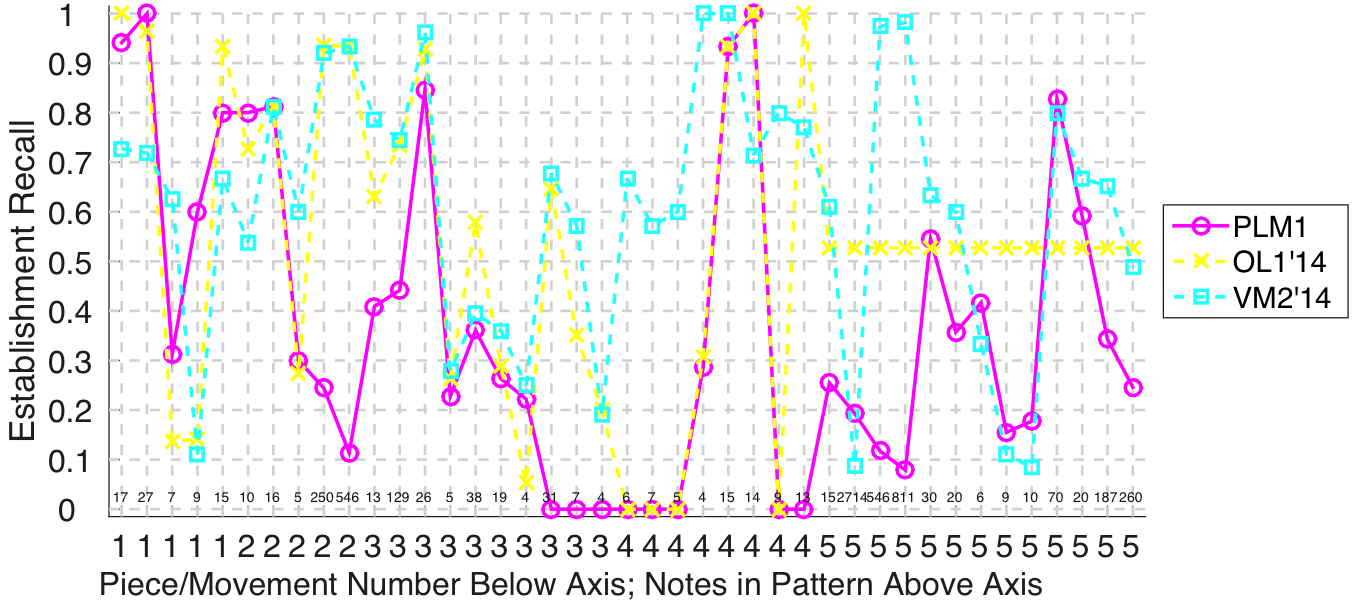
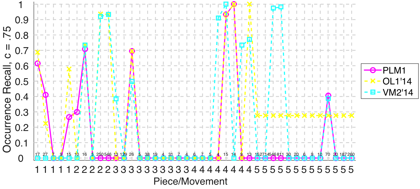
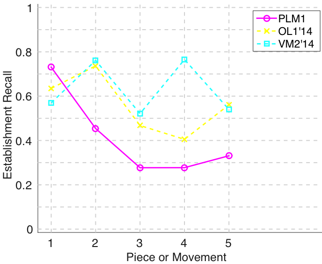
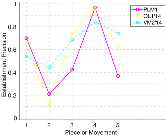
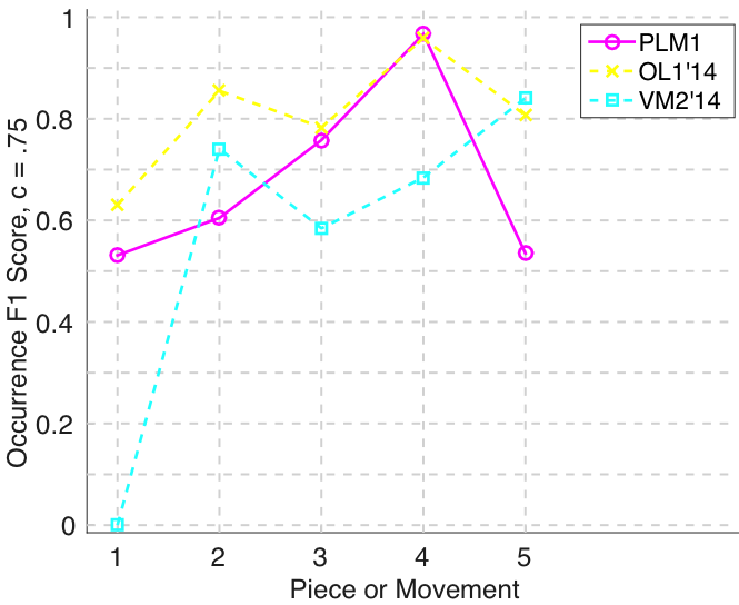
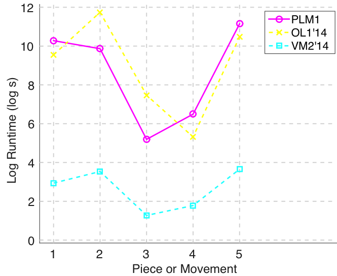
Pesek, Leonardis, and Marolt (2015) submitted a compositional hierarchical model – applied to automatic chord recognition and F0-estimation previously (Pesek, Leonardis, & Marolt, 2014) – to the symMono version of the task. Given that their submission SYMCHM (PLM1) is a general-purpose algorithm for which pattern discovery is one application domain and that this is a popular version of the task (four algorithms submitted in 2014; seven in 2013), SYMCHM (PLM1) did well (Figs. 4-12). It was still not as strong as the previous best performer, VM2 (Velarde & Meredith, 2014), with regards discovering at least one occurrence of each ground truth pattern (Fig. 2): this algorithm, VM2, tested significantly stronger according to Friedman's test than PLM1 (, Bonferroni-corrected). Likewise, it was not as strong as the previous best performer, OL1 (Lartillot, 2014), with regards discovering all occurrences of a given ground truth pattern (Fig. 3): OL1 tested significantly stronger according to Friedman's test than PLM1 (, Bonferroni-corrected), but we should note that the decision to average results for OL1 on piece 5 could be driving this result. It should also be noted that the runtimes for PLM1 (Fig. 13) are somewhat harsh, because the Windows Virtual Machine on which it ran is considerably slower than the Linux machines on which the other submissions ran.
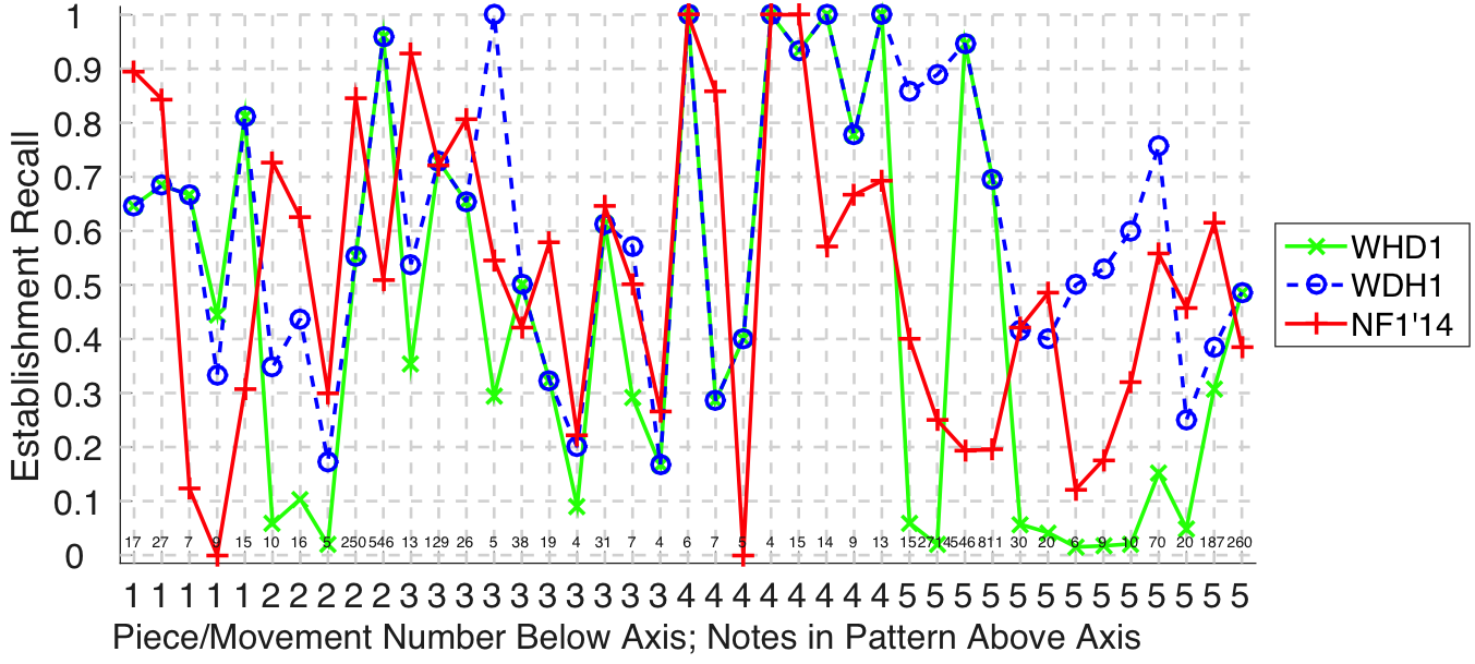
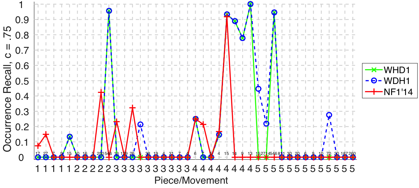
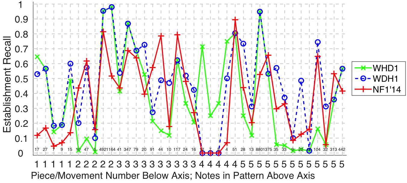
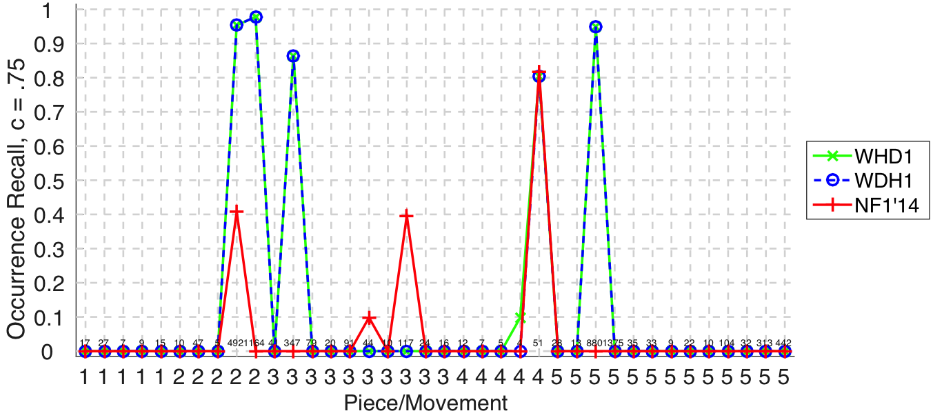
Wang, Hsu, and Dubnov (2015a, 2015b) submitted a motif discovery system based on a Variable Markov Oracle to audMono and audPoly versions of the task. On the audMono task this algorithm, WHD1, was not significantly different to NF1 according to Friedman's test () at discovering at least one occurrence of each ground truth pattern (Fig. 14). Similarly, WHD1 was not significantly different to NF1 according to Friedman's test () at discovering all occurrences of a given ground truth pattern (Fig. 15). These results suggest that WHD1 is on a par with state-of-the-art performance on the audMono task. Results for the audPoly task were similar, and WHD1 was significantly better than previous state-of-the-art performance () with regards discovering at least one occurrence of each ground truth pattern (Fig. 26). (To avoid a bias toward the more numerous submissions of Wang et al. (2015), WHD1 was preselected over WDH1 for comparison with Nieto and Farbood's (2014a) submission, based on performance for the Development Database.)
Discussion
Since this task began in 2013, it has been observed that the discovery of repeated sections tends to be addressed well by submissions, and the discovery of shorter themes/motifs less well. This in itself is not a particularly surprising observation, since it mirrors the way music analysts might agree on the large-scale repetitive structure of a song/piece, but differ in interpreting its themes and/or motifs. It was exciting to see, however, that WDH1 and WHD1 (Wang et al., 2015a, 2015b) had high establishment recall compared with previous years for seven- and nine-note patterns in piece 1, a five-note pattern in piece 2, and nine- and thirteen-note patterns in piece 4 (see Fig. 14 for details). Whereas WHD1's establishment recall dropped off for six- and nine-note patterns in piece 5, establishment recall remained comparatively high for WDH1. The difference between these submissions was a fixed minimum length (FML) criterion that applied to WDH1 but not to WHD1. The criterion seems to have helped WDH1 to perform well on this aspect of the task.
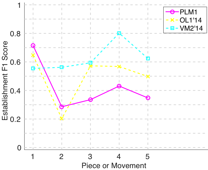
The PLM1 submission (Pesek et al., 2015) is of interest because it (1) is the first deep architecture to be submitted to the task and (2) has been applied to other MIR tasks such as chord and multi-F0 estimation (Pesek et al., 2014). It outperformed previous algorithms on piece 1 (see Figs. 4-6), demonstrating its potential, but had lower establishment recall for pieces 2-5 (see Fig. 4). For those who have called for multipurpose, integrated MIR solutions, this approach represents an encouraging development.
It is good to see submissions from two new groups this year, and that the emphasis the task places on retrieving and evaluating hierarchical structure is being acknowledged and championed elsewhere (McFee, Nieto, & Bello, 2015). Next year we may switch to new training and test databases that focus not directly on the discovery task itself, but on an application of pattern discovery that can be used as a proxy to evaluate the extent to which algorithms have retrieved relevant repetitive material. If you are interested in helping out with the preparation of a new version of the task, you are welcome to get in touch.
Tom Collins, Leicester, 2015
Results in Detail
symMono
(Submission OL1 did not complete on piece 5. The task captain took the decision to assign the mean of the evaluation metrics for OL1 calculated across the remaining pieces.)
Figure 2. Establishment recall on a per-pattern basis. Establishment recall answers the following question. On average, how similar is the most similar algorithm-output pattern to a ground-truth pattern prototype?
Figure 3. Occurrence recall on a per-pattern basis. Occurrence recall answers the following question. On average, how similar is the most similar set of algorithm-output pattern occurrences to a discovered ground-truth occurrence set?
Figure 4. Establishment recall averaged over each piece/movement. Establishment recall answers the following question. On average, how similar is the most similar algorithm-output pattern to a ground-truth pattern prototype?
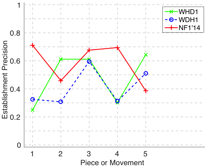
Figure 5. Establishment precision averaged over each piece/movement. Establishment precision answers the following question. On average, how similar is the most similar ground-truth pattern prototype to an algorithm-output pattern?
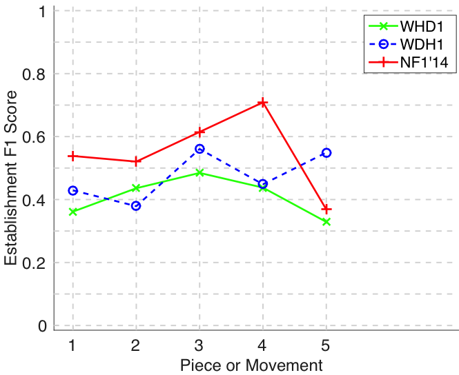
Figure 6. Establishment F1 averaged over each piece/movement. Establishment F1 is an average of establishment precision and establishment recall.
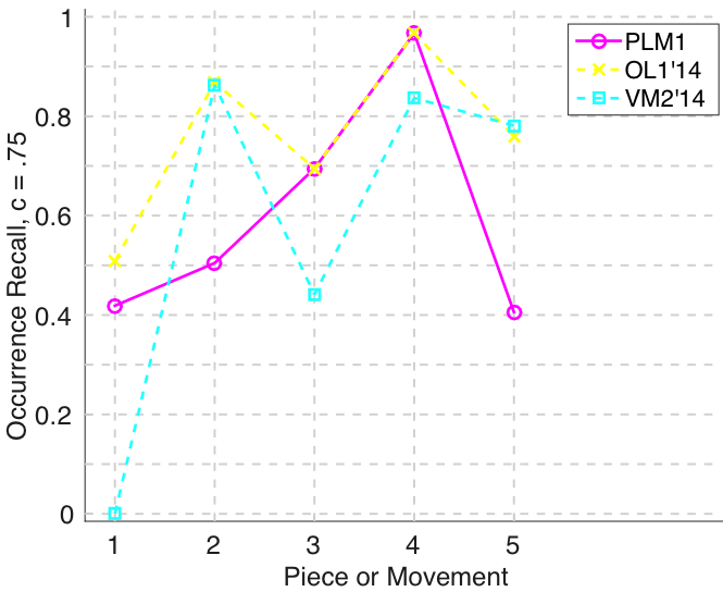
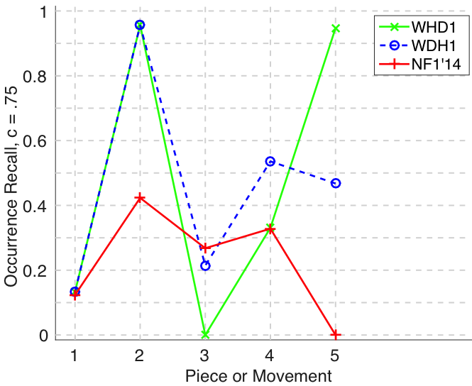
Figure 7. Occurrence recall () averaged over each piece/movement. Occurrence recall answers the following question. On average, how similar is the most similar set of algorithm-output pattern occurrences to a discovered ground-truth occurrence set?
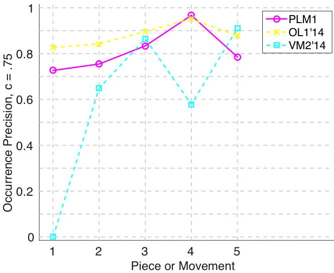
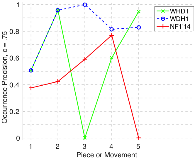
Figure 8. Occurrence precision () averaged over each piece/movement. Occurrence precision answers the following question. On average, how similar is the most similar discovered ground-truth occurrence set to a set of algorithm-output pattern occurrences?
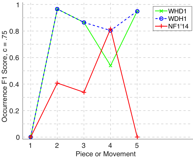
Figure 9. Occurrence F1 () averaged over each piece/movement. Occurrence F1 is an average of occurrence precision and occurrence recall.
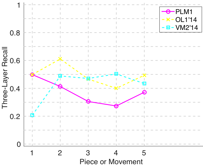
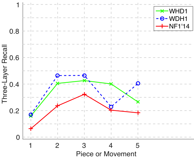
Figure 10. Three-layer recall averaged over each piece/movement. Rather than using as a similarity measure (which is the default for establishment recall), three-layer recall uses , which is a kind of F1 measure.
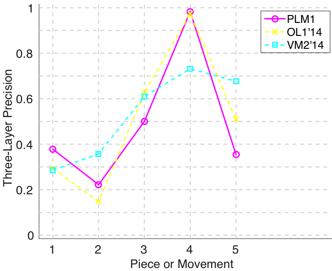
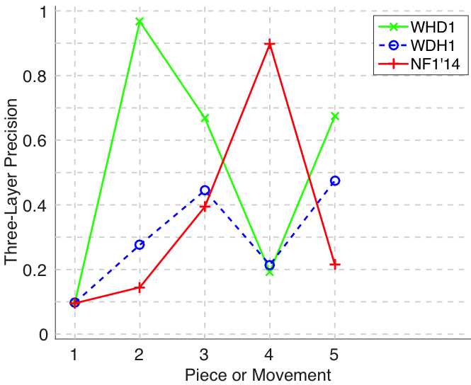
Figure 11. Three-layer precision averaged over each piece/movement. Rather than using as a similarity measure (which is the default for establishment precision), three-layer precision uses , which is a kind of F1 measure.
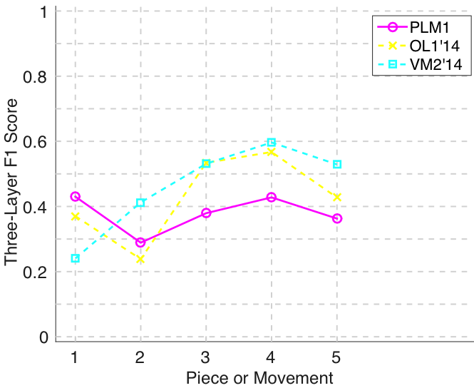
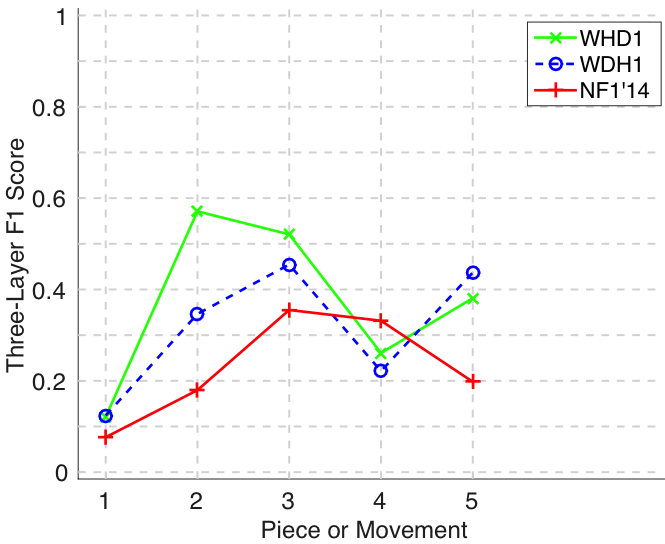
Figure 12. Three-layer F1 (TLF) averaged over each piece/movement. TLF is an average of three-layer precision and three-layer recall.
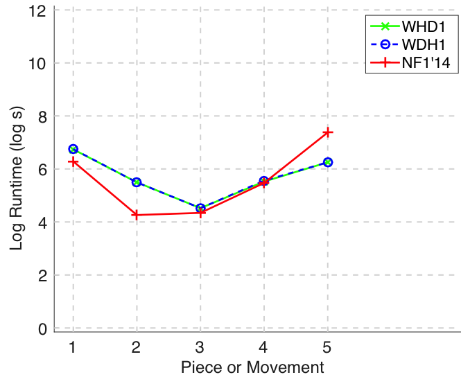
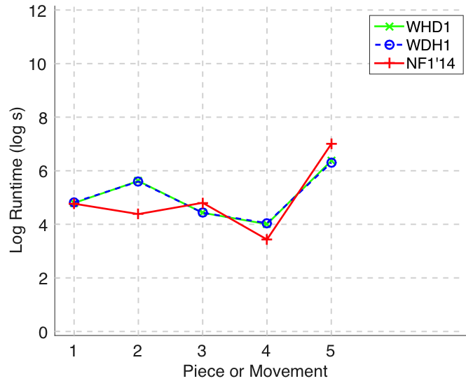
Figure 13. Log runtime of the algorithm for each piece/movement.
audMono
Figure 14. Establishment recall on a per-pattern basis. Establishment recall answers the following question. On average, how similar is the most similar algorithm-output pattern to a ground-truth pattern prototype?
Figure 15. Occurrence recall on a per-pattern basis. Occurrence recall answers the following question. On average, how similar is the most similar set of algorithm-output pattern occurrences to a discovered ground-truth occurrence set?
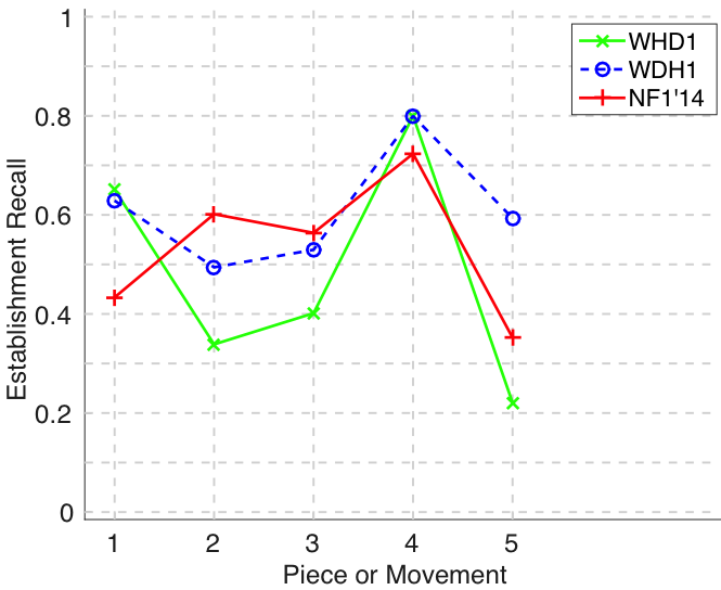
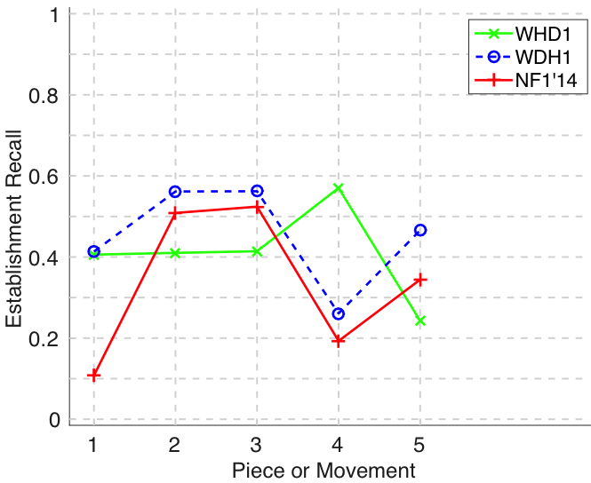
Figure 16. Establishment recall averaged over each piece/movement. Establishment recall answers the following question. On average, how similar is the most similar algorithm-output pattern to a ground-truth pattern prototype?
Figure 17. Establishment precision averaged over each piece/movement. Establishment precision answers the following question. On average, how similar is the most similar ground-truth pattern prototype to an algorithm-output pattern?
Figure 18. Establishment F1 averaged over each piece/movement. Establishment F1 is an average of establishment precision and establishment recall.
Figure 19. Occurrence recall () averaged over each piece/movement. Occurrence recall answers the following question. On average, how similar is the most similar set of algorithm-output pattern occurrences to a discovered ground-truth occurrence set?
Figure 20. Occurrence precision () averaged over each piece/movement. Occurrence precision answers the following question. On average, how similar is the most similar discovered ground-truth occurrence set to a set of algorithm-output pattern occurrences?
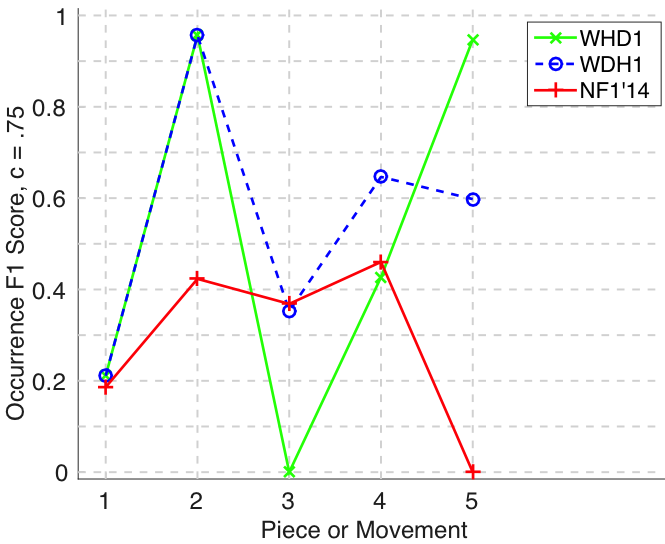
Figure 21. Occurrence F1 () averaged over each piece/movement. Occurrence F1 is an average of occurrence precision and occurrence recall.
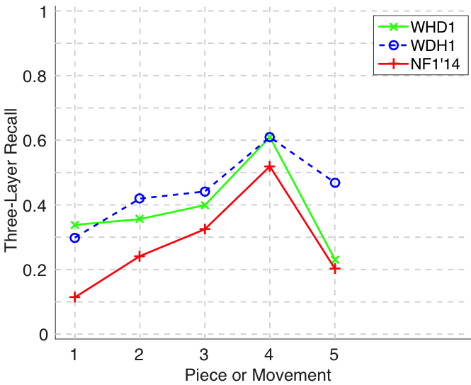
Figure 22. Three-layer recall averaged over each piece/movement. Rather than using as a similarity measure (which is the default for establishment recall), three-layer recall uses , which is a kind of F1 measure.
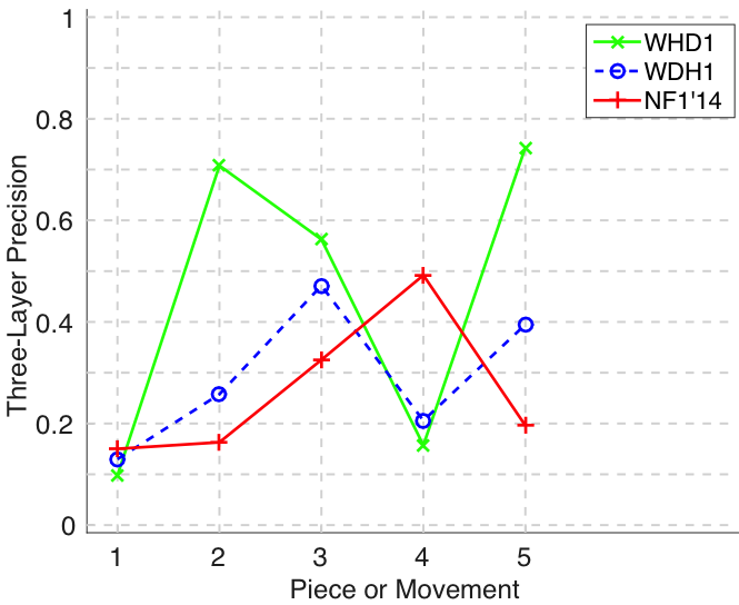
Figure 23. Three-layer precision averaged over each piece/movement. Rather than using as a similarity measure (which is the default for establishment precision), three-layer precision uses , which is a kind of F1 measure.
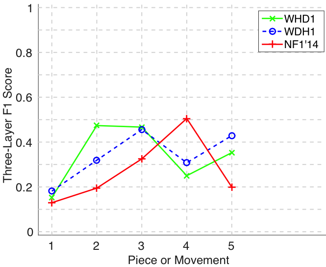
Figure 24. Three-layer F1 (TLF) averaged over each piece/movement. TLF is an average of three-layer precision and three-layer recall.
Figure 25. Log runtime of the algorithm for each piece/movement.
audPoly
Figure 26. Establishment recall on a per-pattern basis. Establishment recall answers the following question. On average, how similar is the most similar algorithm-output pattern to a ground-truth pattern prototype?
Figure 27. Occurrence recall on a per-pattern basis. Occurrence recall answers the following question. On average, how similar is the most similar set of algorithm-output pattern occurrences to a discovered ground-truth occurrence set?
Figure 28. Establishment recall averaged over each piece/movement. Establishment recall answers the following question. On average, how similar is the most similar algorithm-output pattern to a ground-truth pattern prototype?
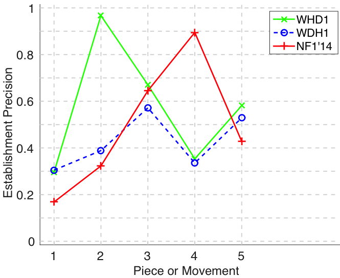
Figure 29. Establishment precision averaged over each piece/movement. Establishment precision answers the following question. On average, how similar is the most similar ground-truth pattern prototype to an algorithm-output pattern?
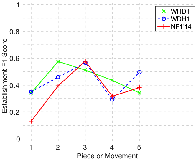
Figure 30. Establishment F1 averaged over each piece/movement. Establishment F1 is an average of establishment precision and establishment recall.
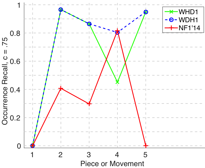
Figure 31. Occurrence recall () averaged over each piece/movement. Occurrence recall answers the following question. On average, how similar is the most similar set of algorithm-output pattern occurrences to a discovered ground-truth occurrence set?
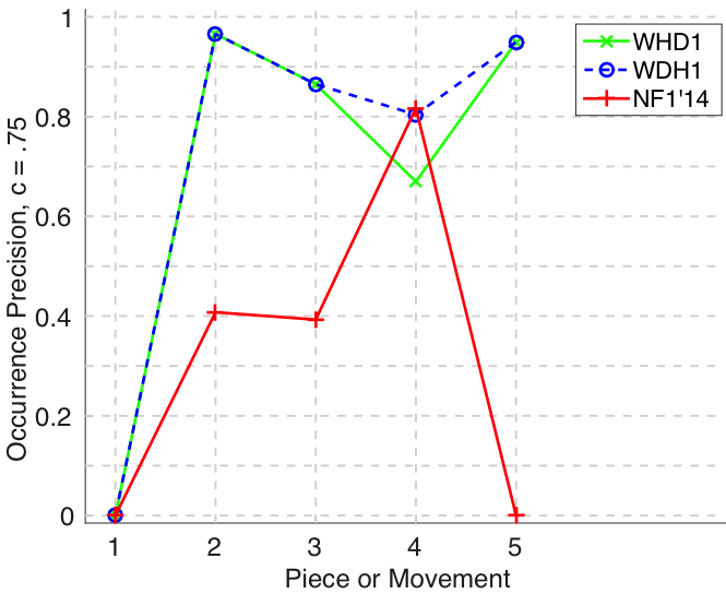
Figure 32. Occurrence precision () averaged over each piece/movement. Occurrence precision answers the following question. On average, how similar is the most similar discovered ground-truth occurrence set to a set of algorithm-output pattern occurrences?
Figure 33. Occurrence F1 () averaged over each piece/movement. Occurrence F1 is an average of occurrence precision and occurrence recall.
Figure 34. Three-layer recall averaged over each piece/movement. Rather than using as a similarity measure (which is the default for establishment recall), three-layer recall uses , which is a kind of F1 measure.
Figure 35. Three-layer precision averaged over each piece/movement. Rather than using as a similarity measure (which is the default for establishment precision), three-layer precision uses , which is a kind of F1 measure.
Figure 36. Three-layer F1 (TLF) averaged over each piece/movement. TLF is an average of three-layer precision and three-layer recall.
Figure 37. Log runtime of the algorithm for each piece/movement.
Tabular Versions of Plots
symMono
| AlgIdx | AlgStub | Piece | n_P | n_Q | P_est | R_est | F1_est | P_occ(c=.75) | R_occ(c=.75) | F_1occ(c=.75) | P_3 | R_3 | TLF_1 | runtime | FRT | FFTP_est | FFP | P_occ(c=.5) | R_occ(c=.5) | F_1occ(c=.5) | P | R | F_1 |
|---|---|---|---|---|---|---|---|---|---|---|---|---|---|---|---|---|---|---|---|---|---|---|---|
| 1 | PLM1 | piece1 | 5 | 18.000 | 0.700 | 0.731 | 0.715 | 0.726 | 0.419 | 0.531 | 0.378 | 0.499 | 0.430 | 29100.000 | 0.000 | 0.480 | 0.294 | 0.579 | 0.433 | 0.495 | 0.000 | 0.000 | 0.000 |
| 1 | PLM1 | piece2 | 5 | 31.000 | 0.209 | 0.454 | 0.286 | 0.755 | 0.505 | 0.605 | 0.222 | 0.413 | 0.289 | 19260.000 | 0.000 | 0.174 | 0.177 | 0.670 | 0.573 | 0.617 | 0.032 | 0.200 | 0.056 |
| 1 | PLM1 | piece3 | 10.000 | 8 | 0.426 | 0.277 | 0.336 | 0.834 | 0.695 | 0.758 | 0.501 | 0.305 | 0.379 | 180.000 | 0.000 | 0.242 | 0.505 | 0.834 | 0.695 | 0.758 | 0.000 | 0.000 | 0.000 |
| 1 | PLM1 | piece4 | 8 | 2 | 0.967 | 0.277 | 0.431 | 0.967 | 0.967 | 0.967 | 0.983 | 0.273 | 0.428 | 660.000 | 0.000 | 0.277 | 0.983 | 0.967 | 0.967 | 0.967 | 0.500 | 0.125 | 0.200 |
| 1 | PLM1 | piece5 | 13.000 | 35.000 | 0.366 | 0.331 | 0.348 | 0.785 | 0.406 | 0.535 | 0.354 | 0.372 | 0.363 | 69240.000 | 0.000 | 0.103 | 0.226 | 0.617 | 0.456 | 0.525 | 0.000 | 0.000 | 0.000 |
| 2 | OL1_14 | piece1 | 5 | 114.000 | 0.660 | 0.635 | 0.647 | 0.827 | 0.509 | 0.630 | 0.295 | 0.498 | 0.370 | 14013.284 | 0.000 | 0.368 | 0.389 | 0.723 | 0.559 | 0.630 | 0.009 | 0.200 | 0.017 |
| 2 | OL1_14 | piece2 | 5 | 98.000 | 0.117 | 0.737 | 0.202 | 0.842 | 0.868 | 0.855 | 0.148 | 0.611 | 0.238 | 126065.856 | 0.000 | 0.277 | 0.440 | 0.750 | 0.709 | 0.729 | 0.020 | 0.400 | 0.039 |
| 2 | OL1_14 | piece3 | 10.000 | 9 | 0.739 | 0.467 | 0.573 | 0.897 | 0.695 | 0.783 | 0.625 | 0.466 | 0.534 | 1751.959 | 0.000 | 0.348 | 0.622 | 0.728 | 0.608 | 0.663 | 0.111 | 0.100 | 0.105 |
| 2 | OL1_14 | piece4 | 8 | 4 | 0.950 | 0.405 | 0.568 | 0.950 | 0.967 | 0.958 | 0.974 | 0.400 | 0.567 | 204.197 | 0.000 | 0.405 | 0.974 | 0.950 | 0.967 | 0.958 | 0.500 | 0.250 | 0.333 |
| 2 | OL1_14 | piece5 | 13.000 | 56.250 | 0.617 | 0.561 | 0.498 | 0.879 | 0.760 | 0.807 | 0.510 | 0.494 | 0.427 | 35508.820 | 0.000 | 0.350 | 0.606 | 0.788 | 0.711 | 0.745 | 0.160 | 0.237 | 0.124 |
| 3 | VM2_14 | piece1 | 5 | 5 | 0.540 | 0.570 | 0.555 | 0.000 | 0.000 | 0.000 | 0.286 | 0.207 | 0.240 | 18.906 | 0.000 | 0.570 | 0.286 | 0.291 | 0.490 | 0.365 | 0.000 | 0.000 | 0.000 |
| 3 | VM2_14 | piece2 | 5 | 7 | 0.446 | 0.761 | 0.562 | 0.649 | 0.863 | 0.741 | 0.357 | 0.488 | 0.413 | 34.308 | 0.000 | 0.419 | 0.128 | 0.427 | 0.630 | 0.509 | 0.143 | 0.200 | 0.167 |
| 3 | VM2_14 | piece3 | 10.000 | 7 | 0.690 | 0.521 | 0.594 | 0.865 | 0.441 | 0.584 | 0.609 | 0.471 | 0.531 | 3.570 | 0.000 | 0.393 | 0.541 | 0.662 | 0.561 | 0.607 | 0.000 | 0.000 | 0.000 |
| 3 | VM2_14 | piece4 | 8 | 6 | 0.842 | 0.765 | 0.802 | 0.579 | 0.837 | 0.684 | 0.732 | 0.504 | 0.597 | 5.942 | 0.000 | 0.721 | 0.711 | 0.410 | 0.732 | 0.525 | 0.167 | 0.125 | 0.143 |
| 3 | VM2_14 | piece5 | 13.000 | 7 | 0.739 | 0.540 | 0.624 | 0.910 | 0.781 | 0.841 | 0.677 | 0.434 | 0.529 | 38.698 | 0.000 | 0.420 | 0.554 | 0.517 | 0.636 | 0.570 | 0.000 | 0.000 | 0.000 |
Table 2. Tabular version of Figures 4-13.
| AlgIdx | AlgStub | Piece | n_P | R_est | R_occ(c=.75) | R_occ(c=.5) | ||||||
|---|---|---|---|---|---|---|---|---|---|---|---|---|
| 1 | PLM1 | piece1 | 5 | |||||||||
| 0.941 | 1.000 | 0.312 | 0.600 | 0.800 | ||||||||
| 0.614 | 0.410 | 0.000 | 0.000 | 0.267 | ||||||||
| 0.614 | 0.410 | 0.000 | 0.000 | 0.267 | ||||||||
| 1 | PLM1 | piece2 | 5 | |||||||||
| 0.800 | 0.812 | 0.300 | 0.244 | 0.114 | ||||||||
| 0.300 | 0.709 | 0.000 | 0.000 | 0.000 | ||||||||
| 0.300 | 0.709 | 0.000 | 0.000 | 0.000 | ||||||||
| 1 | PLM1 | piece3 | 10.000 | |||||||||
| 0.409 | 0.442 | 0.846 | 0.227 | 0.361 | 0.263 | 0.222 | 0.000 | 0.000 | 0.000 | |||
| 0.00000 | 0.000 | 0.695 | 0.000 | 0.000 | 0.000 | 0.000 | 0.000 | 0.000 | 0.000 | |||
| 0.00000 | 0.000 | 0.695 | 0.000 | 0.000 | 0.000 | 0.000 | 0.000 | 0.000 | 0.000 | |||
| 1 | PLM1 | piece4 | 8 | |||||||||
| 0.00000 | 0.000 | 0.000 | 0.286 | 0.933 | 1.000 | 0.000 | 0.000 | |||||
| 0.00000 | 0.000 | 0.000 | 0.000 | 0.933 | 1.000 | 0.000 | 0.000 | |||||
| 0.00000 | 0.000 | 0.000 | 0.000 | 0.933 | 1.000 | 0.000 | 0.000 | |||||
| 1 | PLM1 | piece5 | 13.000 | |||||||||
| 0.255 | 0.193 | 0.117 | 0.079 | 0.545 | 0.357 | 0.417 | 0.155 | 0.177 | 0.829 | 0.591 | 0.342 | 0.246 |
| 0.00000 | 0.000 | 0.000 | 0.000 | 0.000 | 0.000 | 0.000 | 0.000 | 0.000 | 0.406 | 0.000 | 0.000 | 0.000 |
| 0.00000 | 0.000 | 0.000 | 0.000 | 0.000 | 0.000 | 0.000 | 0.000 | 0.000 | 0.406 | 0.000 | 0.000 | 0.000 |
| 2 | OL1_14 | piece1 | 5 | |||||||||
| 1.00000 | 0.964 | 0.137 | 0.140 | 0.933 | ||||||||
| 0.688 | 0.226 | 0.000 | 0.000 | 0.578 | ||||||||
| 0.688 | 0.226 | 0.000 | 0.000 | 0.578 | ||||||||
| 2 | OL1_14 | piece2 | 5 | |||||||||
| 0.727 | 0.812 | 0.273 | 0.936 | 0.934 | ||||||||
| 0.00000 | 0.734 | 0.000 | 0.936 | 0.934 | ||||||||
| 0.00000 | 0.734 | 0.000 | 0.936 | 0.934 | ||||||||
| 2 | OL1_14 | piece3 | 10.000 | |||||||||
| 0.632 | 0.735 | 0.929 | 0.263 | 0.579 | 0.289 | 0.053 | 0.645 | 0.350 | 0.200 | |||
| 0.00000 | 0.000 | 0.695 | 0.000 | 0.000 | 0.000 | 0.000 | 0.000 | 0.000 | 0.000 | |||
| 0.00000 | 0.000 | 0.695 | 0.000 | 0.000 | 0.000 | 0.000 | 0.000 | 0.000 | 0.000 | |||
| 2 | OL1_14 | piece4 | 8 | |||||||||
| 0.00000 | 0.000 | 0.000 | 0.308 | 0.933 | 1.000 | 0.000 | 1.000 | |||||
| 0.00000 | 0.000 | 0.000 | 0.000 | 0.933 | 1.000 | 0.000 | 1.000 | |||||
| 0.00000 | 0.000 | 0.000 | 0.000 | 0.933 | 1.000 | 0.000 | 1.000 | |||||
| 2 | OL1_14 | piece5 | 13.000 | |||||||||
| 0.528 | 0.528 | 0.528 | 0.528 | 0.528 | 0.528 | 0.528 | 0.528 | 0.528 | 0.528 | 0.528 | 0.528 | 0.528 |
| 0.276 | 0.276 | 0.276 | 0.276 | 0.276 | 0.276 | 0.276 | 0.276 | 0.276 | 0.276 | 0.276 | 0.276 | 0.276 |
| 0.276 | 0.276 | 0.276 | 0.276 | 0.276 | 0.276 | 0.276 | 0.276 | 0.276 | 0.276 | 0.276 | 0.276 | 0.276 |
| 3 | VM2_14 | piece1 | 5 | |||||||||
| 0.727 | 0.719 | 0.625 | 0.111 | 0.667 | ||||||||
| 0.00000 | 0.000 | 0.000 | 0.000 | 0.000 | ||||||||
| 0.00000 | 0.000 | 0.000 | 0.000 | 0.000 | ||||||||
| 3 | VM2_14 | piece2 | 5 | |||||||||
| 0.538 | 0.812 | 0.600 | 0.920 | 0.934 | ||||||||
| 0.00000 | 0.734 | 0.000 | 0.920 | 0.934 | ||||||||
| 0.00000 | 0.734 | 0.000 | 0.920 | 0.934 | ||||||||
| 3 | VM2_14 | piece3 | 10.000 | |||||||||
| 0.786 | 0.744 | 0.962 | 0.278 | 0.395 | 0.360 | 0.250 | 0.677 | 0.571 | 0.190 | |||
| 0.384 | 0.000 | 0.498 | 0.000 | 0.000 | 0.000 | 0.000 | 0.000 | 0.000 | 0.000 | |||
| 0.384 | 0.000 | 0.498 | 0.000 | 0.000 | 0.000 | 0.000 | 0.000 | 0.000 | 0.000 | |||
| 3 | VM2_14 | piece4 | 8 | |||||||||
| 0.667 | 0.571 | 0.600 | 1.000 | 1.000 | 0.714 | 0.800 | 0.769 | |||||
| 0.00000 | 0.000 | 0.000 | 0.911 | 1.000 | 0.000 | 0.733 | 0.769 | |||||
| 0.00000 | 0.000 | 0.000 | 0.911 | 1.000 | 0.000 | 0.733 | 0.769 | |||||
| 3 | VM2_14 | piece5 | 13.000 | |||||||||
| 0.609 | 0.087 | 0.974 | 0.982 | 0.633 | 0.600 | 0.333 | 0.111 | 0.084 | 0.800 | 0.667 | 0.652 | 0.488 |
| 0.00000 | 0.000 | 0.974 | 0.982 | 0.000 | 0.000 | 0.000 | 0.000 | 0.000 | 0.388 | 0.000 | 0.000 | 0.000 |
| 0.00000 | 0.000 | 0.974 | 0.982 | 0.000 | 0.000 | 0.000 | 0.000 | 0.000 | 0.388 | 0.000 | 0.000 | 0.000 |
Table 3. Tabular version of Figures 2 and 3.
audMono
| AlgIdx | AlgStub | Piece | n_P | n_Q | P_est | R_est | F1_est | P_occ(c=.75) | R_occ(c=.75) | F_1occ(c=.75) | P_3 | R_3 | TLF_1 | runtime | FRT | FFTP_est | FFP | P_occ(c=.5) | R_occ(c=.5) | F_1occ(c=.5) | P | R | F_1 |
|---|---|---|---|---|---|---|---|---|---|---|---|---|---|---|---|---|---|---|---|---|---|---|---|
| 1 | WHD1 | piece1 | 5 | 131.000 | 0.250 | 0.651 | 0.362 | 0.506 | 0.133 | 0.211 | 0.098 | 0.338 | 0.152 | 845.000 | 0.000 | 0.089 | 0.112 | 0.416 | 0.213 | 0.282 | 0.000 | 0.000 | 0.000 |
| 1 | WHD1 | piece2 | 5 | 3 | 0.612 | 0.339 | 0.436 | 0.956 | 0.956 | 0.956 | 0.708 | 0.356 | 0.474 | 244.000 | 0.000 | 0.339 | 0.708 | 0.754 | 0.754 | 0.754 | 0.000 | 0.000 | 0.000 |
| 1 | WHD1 | piece3 | 10.000 | 7 | 0.611 | 0.402 | 0.485 | 0.000 | 0.000 | 0.000 | 0.562 | 0.399 | 0.467 | 92.000 | 0.000 | 0.344 | 0.551 | 0.603 | 0.486 | 0.538 | 0.000 | 0.000 | 0.000 |
| 1 | WHD1 | piece4 | 8 | 88.000 | 0.301 | 0.800 | 0.438 | 0.601 | 0.331 | 0.427 | 0.157 | 0.609 | 0.250 | 251.000 | 0.000 | 0.257 | 0.278 | 0.523 | 0.291 | 0.373 | 0.023 | 0.250 | 0.042 |
| 1 | WHD1 | piece5 | 13.000 | 3 | 0.644 | 0.221 | 0.329 | 0.947 | 0.947 | 0.947 | 0.743 | 0.231 | 0.353 | 519.000 | 0.000 | 0.221 | 0.743 | 0.821 | 0.821 | 0.821 | 0.000 | 0.000 | 0.000 |
| 2 | WDH1 | piece1 | 5 | 56.000 | 0.326 | 0.629 | 0.429 | 0.506 | 0.133 | 0.211 | 0.130 | 0.299 | 0.181 | 852.000 | 0.000 | 0.436 | 0.240 | 0.464 | 0.203 | 0.283 | 0.000 | 0.000 | 0.000 |
| 2 | WDH1 | piece2 | 5 | 11.000 | 0.307 | 0.494 | 0.379 | 0.956 | 0.956 | 0.956 | 0.258 | 0.419 | 0.319 | 243.000 | 0.000 | 0.317 | 0.268 | 0.754 | 0.754 | 0.754 | 0.000 | 0.000 | 0.000 |
| 2 | WDH1 | piece3 | 10.000 | 13.000 | 0.596 | 0.530 | 0.561 | 1.000 | 0.214 | 0.353 | 0.471 | 0.441 | 0.456 | 92.000 | 0.000 | 0.265 | 0.475 | 0.538 | 0.381 | 0.446 | 0.000 | 0.000 | 0.000 |
| 2 | WDH1 | piece4 | 8 | 45.000 | 0.312 | 0.800 | 0.448 | 0.815 | 0.536 | 0.647 | 0.206 | 0.609 | 0.308 | 259.000 | 0.000 | 0.208 | 0.247 | 0.706 | 0.458 | 0.555 | 0.044 | 0.250 | 0.075 |
| 2 | WDH1 | piece5 | 13.000 | 23.000 | 0.511 | 0.593 | 0.549 | 0.829 | 0.468 | 0.598 | 0.395 | 0.469 | 0.429 | 518.000 | 0.000 | 0.251 | 0.444 | 0.663 | 0.355 | 0.462 | 0.000 | 0.000 | 0.000 |
| 3 | NF1_14 | piece1 | 5 | 5 | 0.710 | 0.433 | 0.538 | 0.375 | 0.124 | 0.186 | 0.150 | 0.114 | 0.129 | 536.000 | 0.000 | 0.433 | 0.150 | 0.344 | 0.130 | 0.189 | 0.000 | 0.000 | 0.000 |
| 3 | NF1_14 | piece2 | 5 | 12.000 | 0.459 | 0.602 | 0.520 | 0.423 | 0.423 | 0.423 | 0.163 | 0.242 | 0.195 | 71.000 | 0.000 | 0.351 | 0.171 | 0.457 | 0.187 | 0.266 | 0.000 | 0.000 | 0.000 |
| 3 | NF1_14 | piece3 | 10.000 | 17.000 | 0.676 | 0.564 | 0.615 | 0.590 | 0.268 | 0.368 | 0.325 | 0.325 | 0.325 | 77.000 | 0.000 | 0.429 | 0.376 | 0.428 | 0.260 | 0.323 | 0.000 | 0.000 | 0.000 |
| 3 | NF1_14 | piece4 | 8 | 13.000 | 0.695 | 0.723 | 0.709 | 0.770 | 0.328 | 0.460 | 0.492 | 0.519 | 0.505 | 238.000 | 0.000 | 0.330 | 0.398 | 0.664 | 0.379 | 0.482 | 0.077 | 0.125 | 0.095 |
| 3 | NF1_14 | piece5 | 13.000 | 23.000 | 0.387 | 0.352 | 0.369 | 0.000 | 0.000 | 0.000 | 0.196 | 0.203 | 0.199 | 1598.000 | 0.000 | 0.258 | 0.218 | 0.365 | 0.147 | 0.210 | 0.000 | 0.000 | 0.000 |
Table 4. Taublar version of Figures 16-25.
| AlgIdx | AlgStub | Piece | n_P | R_est | R_occ(c=.75) | R_occ(c=.5) | ||||||
|---|---|---|---|---|---|---|---|---|---|---|---|---|
| 1 | WHD1 | piece1 | 5 | |||||||||
| 0.647 | 0.684 | 0.667 | 0.444 | 0.812 | ||||||||
| 0.00000 | 0.000 | 0.000 | 0.000 | 0.133 | ||||||||
| 0.00000 | 0.000 | 0.000 | 0.000 | 0.133 | ||||||||
| 1 | WHD1 | piece2 | 5 | |||||||||
| 0.058 | 0.104 | 0.019 | 0.552 | 0.960 | ||||||||
| 0.00000 | 0.000 | 0.000 | 0.000 | 0.956 | ||||||||
| 0.00000 | 0.000 | 0.000 | 0.000 | 0.956 | ||||||||
| 1 | WHD1 | piece3 | 10.000 | |||||||||
| 0.353 | 0.729 | 0.654 | 0.294 | 0.500 | 0.324 | 0.091 | 0.613 | 0.292 | 0.167 | |||
| 0.00000 | 0.000 | 0.000 | 0.000 | 0.000 | 0.000 | 0.000 | 0.000 | 0.000 | 0.000 | |||
| 0.00000 | 0.000 | 0.000 | 0.000 | 0.000 | 0.000 | 0.000 | 0.000 | 0.000 | 0.000 | |||
| 1 | WHD1 | piece4 | 8 | |||||||||
| 1.00000 | 0.286 | 0.400 | 1.000 | 0.933 | 1.000 | 0.778 | 1.000 | |||||
| 0.250 | 0.000 | 0.000 | 0.146 | 0.933 | 0.889 | 0.778 | 1.000 | |||||
| 0.250 | 0.000 | 0.000 | 0.146 | 0.933 | 0.889 | 0.778 | 1.000 | |||||
| 1 | WHD1 | piece5 | 13.000 | |||||||||
| 0.060 | 0.019 | 0.947 | 0.697 | 0.057 | 0.042 | 0.015 | 0.017 | 0.021 | 0.152 | 0.049 | 0.308 | 0.487 |
| 0.00000 | 0.000 | 0.947 | 0.000 | 0.000 | 0.000 | 0.000 | 0.000 | 0.000 | 0.000 | 0.000 | 0.000 | 0.000 |
| 0.00000 | 0.000 | 0.947 | 0.000 | 0.000 | 0.000 | 0.000 | 0.000 | 0.000 | 0.000 | 0.000 | 0.000 | 0.000 |
| 2 | WDH1 | piece1 | 5 | |||||||||
| 0.647 | 0.684 | 0.667 | 0.333 | 0.812 | ||||||||
| 0.00000 | 0.000 | 0.000 | 0.000 | 0.133 | ||||||||
| 0.00000 | 0.000 | 0.000 | 0.000 | 0.133 | ||||||||
| 2 | WDH1 | piece2 | 5 | |||||||||
| 0.348 | 0.438 | 0.174 | 0.552 | 0.960 | ||||||||
| 0.00000 | 0.000 | 0.000 | 0.000 | 0.956 | ||||||||
| 0.00000 | 0.000 | 0.000 | 0.000 | 0.956 | ||||||||
| 2 | WDH1 | piece3 | 10.000 | |||||||||
| 0.538 | 0.729 | 0.654 | 1.000 | 0.500 | 0.324 | 0.200 | 0.613 | 0.571 | 0.167 | |||
| 0.00000 | 0.000 | 0.000 | 0.214 | 0.000 | 0.000 | 0.000 | 0.000 | 0.000 | 0.000 | |||
| 0.00000 | 0.000 | 0.000 | 0.214 | 0.000 | 0.000 | 0.000 | 0.000 | 0.000 | 0.000 | |||
| 2 | WDH1 | piece4 | 8 | |||||||||
| 1.00000 | 0.286 | 0.400 | 1.000 | 0.933 | 1.000 | 0.778 | 1.000 | |||||
| 0.250 | 0.000 | 0.000 | 0.146 | 0.933 | 0.889 | 0.778 | 1.000 | |||||
| 0.250 | 0.000 | 0.000 | 0.146 | 0.933 | 0.889 | 0.778 | 1.000 | |||||
| 2 | WDH1 | piece5 | 13.000 | |||||||||
| 0.857 | 0.889 | 0.947 | 0.697 | 0.417 | 0.400 | 0.500 | 0.529 | 0.600 | 0.757 | 0.250 | 0.385 | 0.487 |
| 0.446 | 0.220 | 0.947 | 0.000 | 0.000 | 0.000 | 0.000 | 0.000 | 0.000 | 0.277 | 0.000 | 0.000 | 0.000 |
| 0.446 | 0.220 | 0.947 | 0.000 | 0.000 | 0.000 | 0.000 | 0.000 | 0.000 | 0.277 | 0.000 | 0.000 | 0.000 |
| 3 | NF1_14 | piece1 | 5 | |||||||||
| 0.895 | 0.844 | 0.123 | 0.000 | 0.306 | ||||||||
| 0.075 | 0.148 | 0.000 | 0.000 | 0.000 | ||||||||
| 0.075 | 0.148 | 0.000 | 0.000 | 0.000 | ||||||||
| 3 | NF1_14 | piece2 | 5 | |||||||||
| 0.727 | 0.625 | 0.300 | 0.846 | 0.509 | ||||||||
| 0.00000 | 0.000 | 0.000 | 0.423 | 0.000 | ||||||||
| 0.00000 | 0.000 | 0.000 | 0.423 | 0.000 | ||||||||
| 3 | NF1_14 | piece3 | 10.000 | |||||||||
| 0.929 | 0.721 | 0.808 | 0.545 | 0.421 | 0.579 | 0.222 | 0.645 | 0.500 | 0.267 | |||
| 0.231 | 0.000 | 0.322 | 0.000 | 0.000 | 0.000 | 0.000 | 0.000 | 0.000 | 0.000 | |||
| 0.231 | 0.000 | 0.322 | 0.000 | 0.000 | 0.000 | 0.000 | 0.000 | 0.000 | 0.000 | |||
| 3 | NF1_14 | piece4 | 8 | |||||||||
| 1.00000 | 0.857 | 0.000 | 1.000 | 1.000 | 0.571 | 0.667 | 0.692 | |||||
| 0.250 | 0.214 | 0.000 | 0.167 | 0.917 | 0.000 | 0.000 | 0.000 | |||||
| 0.250 | 0.214 | 0.000 | 0.167 | 0.917 | 0.000 | 0.000 | 0.000 | |||||
| 3 | NF1_14 | piece5 | 13.000 | |||||||||
| 0.400 | 0.250 | 0.194 | 0.195 | 0.421 | 0.485 | 0.121 | 0.176 | 0.321 | 0.557 | 0.457 | 0.615 | 0.385 |
| 0.00000 | 0.000 | 0.000 | 0.000 | 0.000 | 0.000 | 0.000 | 0.000 | 0.000 | 0.000 | 0.000 | 0.000 | 0.000 |
| 0.00000 | 0.000 | 0.000 | 0.000 | 0.000 | 0.000 | 0.000 | 0.000 | 0.000 | 0.000 | 0.000 | 0.000 | 0.000 |
Table 5. Tabular version of Figures 14 and 15.
audPoly
| AlgIdx | AlgStub | Piece | n_P | n_Q | P_est | R_est | F1_est | P_occ(c=.75) | R_occ(c=.75) | F_1occ(c=.75) | P_3 | R_3 | TLF_1 | runtime | FRT | FFTP_est | FFP | P_occ(c=.5) | R_occ(c=.5) | F_1occ(c=.5) | P | R | F_1 |
|---|---|---|---|---|---|---|---|---|---|---|---|---|---|---|---|---|---|---|---|---|---|---|---|
| 1 | WHD1 | piece1 | 5 | 89.000 | 0.296 | 0.406 | 0.342 | 0.000 | 0.000 | 0.000 | 0.098 | 0.160 | 0.121 | 121.000 | 0.000 | 0.200 | 0.118 | 0.399 | 0.091 | 0.148 | 0.000 | 0.000 | 0.000 |
| 1 | WHD1 | piece2 | 5 | 2 | 0.967 | 0.410 | 0.576 | 0.966 | 0.966 | 0.966 | 0.967 | 0.405 | 0.571 | 275.000 | 0.000 | 0.410 | 0.967 | 0.966 | 0.966 | 0.966 | 0.000 | 0.000 | 0.000 |
| 1 | WHD1 | piece3 | 10.000 | 5 | 0.670 | 0.414 | 0.512 | 0.865 | 0.865 | 0.865 | 0.668 | 0.426 | 0.521 | 84.000 | 0.000 | 0.414 | 0.668 | 0.664 | 0.511 | 0.577 | 0.000 | 0.000 | 0.000 |
| 1 | WHD1 | piece4 | 5 | 33.000 | 0.353 | 0.570 | 0.436 | 0.670 | 0.451 | 0.539 | 0.193 | 0.401 | 0.261 | 55.000 | 0.000 | 0.311 | 0.313 | 0.506 | 0.264 | 0.347 | 0.000 | 0.000 | 0.000 |
| 1 | WHD1 | piece5 | 13.000 | 4 | 0.581 | 0.243 | 0.342 | 0.950 | 0.950 | 0.950 | 0.675 | 0.265 | 0.381 | 584.000 | 0.000 | 0.243 | 0.675 | 0.686 | 0.585 | 0.631 | 0.000 | 0.000 | 0.000 |
| 2 | WDH1 | piece1 | 5 | 110.000 | 0.305 | 0.413 | 0.351 | 0.000 | 0.000 | 0.000 | 0.097 | 0.170 | 0.124 | 124.000 | 0.000 | 0.200 | 0.118 | 0.354 | 0.109 | 0.167 | 0.000 | 0.000 | 0.000 |
| 2 | WDH1 | piece2 | 5 | 10.000 | 0.389 | 0.562 | 0.459 | 0.966 | 0.966 | 0.966 | 0.276 | 0.464 | 0.346 | 270.000 | 0.000 | 0.281 | 0.247 | 0.600 | 0.523 | 0.559 | 0.000 | 0.000 | 0.000 |
| 2 | WDH1 | piece3 | 10.000 | 14.000 | 0.572 | 0.562 | 0.567 | 0.865 | 0.865 | 0.865 | 0.445 | 0.465 | 0.455 | 84.000 | 0.000 | 0.356 | 0.566 | 0.521 | 0.356 | 0.423 | 0.000 | 0.000 | 0.000 |
| 2 | WDH1 | piece4 | 5 | 7 | 0.335 | 0.261 | 0.293 | 0.804 | 0.804 | 0.804 | 0.214 | 0.229 | 0.221 | 57.000 | 0.000 | 0.261 | 0.300 | 0.589 | 0.444 | 0.506 | 0.000 | 0.000 | 0.000 |
| 2 | WDH1 | piece5 | 13.000 | 16.000 | 0.529 | 0.466 | 0.495 | 0.950 | 0.950 | 0.950 | 0.475 | 0.405 | 0.437 | 545.000 | 0.000 | 0.253 | 0.493 | 0.674 | 0.453 | 0.542 | 0.000 | 0.000 | 0.000 |
| 3 | NF1_14 | piece1 | 5 | 1 | 0.168 | 0.108 | 0.132 | 0.000 | 0.000 | 0.000 | 0.095 | 0.064 | 0.076 | 118.000 | 0.000 | 0.108 | 0.095 | 0.000 | 0.000 | 0.000 | 0.000 | 0.000 | 0.000 |
| 3 | NF1_14 | piece2 | 5 | 12.000 | 0.323 | 0.509 | 0.395 | 0.408 | 0.408 | 0.408 | 0.145 | 0.236 | 0.180 | 80.000 | 0.000 | 0.410 | 0.254 | 0.493 | 0.288 | 0.363 | 0.000 | 0.000 | 0.000 |
| 3 | NF1_14 | piece3 | 10.000 | 10.000 | 0.645 | 0.524 | 0.578 | 0.393 | 0.297 | 0.338 | 0.394 | 0.323 | 0.355 | 122.000 | 0.000 | 0.354 | 0.399 | 0.438 | 0.285 | 0.345 | 0.000 | 0.000 | 0.000 |
| 3 | NF1_14 | piece4 | 5 | 1 | 0.895 | 0.193 | 0.317 | 0.817 | 0.817 | 0.817 | 0.897 | 0.203 | 0.332 | 31.000 | 0.000 | 0.193 | 0.897 | 0.817 | 0.817 | 0.817 | 0.000 | 0.000 | 0.000 |
| 3 | NF1_14 | piece5 | 13.000 | 12.000 | 0.428 | 0.344 | 0.382 | 0.000 | 0.000 | 0.000 | 0.215 | 0.183 | 0.198 | 1096.000 | 0.000 | 0.303 | 0.243 | 0.362 | 0.200 | 0.258 | 0.000 | 0.000 | 0.000 |
Table 8. Tabular version of Figures 28-37.
| AlgIdx | AlgStub | Piece | n_P | R_est | R_occ(c=.75) | R_occ(c=.5) | ||||||
|---|---|---|---|---|---|---|---|---|---|---|---|---|
| 1 | WHD1 | piece1 | 5 | |||||||||
| 0.647 | 0.567 | 0.143 | 0.189 | 0.484 | ||||||||
| 0.00000 | 0.000 | 0.000 | 0.000 | 0.000 | ||||||||
| 0.00000 | 0.000 | 0.000 | 0.000 | 0.000 | ||||||||
| 1 | WHD1 | piece2 | 5 | |||||||||
| 0.016 | 0.095 | 0.006 | 0.953 | 0.980 | ||||||||
| 0.00000 | 0.000 | 0.000 | 0.953 | 0.978 | ||||||||
| 0.00000 | 0.000 | 0.000 | 0.953 | 0.978 | ||||||||
| 1 | WHD1 | piece3 | 10.000 | |||||||||
| 0.415 | 0.869 | 0.688 | 0.526 | 0.214 | 0.149 | 0.119 | 0.624 | 0.333 | 0.205 | |||
| 0.00000 | 0.865 | 0.000 | 0.000 | 0.000 | 0.000 | 0.000 | 0.000 | 0.000 | 0.000 | |||
| 0.00000 | 0.865 | 0.000 | 0.000 | 0.000 | 0.000 | 0.000 | 0.000 | 0.000 | 0.000 | |||
| 1 | WHD1 | piece4 | 5 | |||||||||
| 0.714 | 0.250 | 0.333 | 0.750 | 0.804 | ||||||||
| 0.00000 | 0.000 | 0.000 | 0.098 | 0.804 | ||||||||
| 0.00000 | 0.000 | 0.000 | 0.098 | 0.804 | ||||||||
| 1 | WHD1 | piece5 | 13.000 | |||||||||
| 0.250 | 0.118 | 0.950 | 0.533 | 0.056 | 0.050 | 0.015 | 0.024 | 0.015 | 0.162 | 0.056 | 0.360 | 0.566 |
| 0.00000 | 0.000 | 0.950 | 0.000 | 0.000 | 0.000 | 0.000 | 0.000 | 0.000 | 0.000 | 0.000 | 0.000 | 0.000 |
| 0.00000 | 0.000 | 0.950 | 0.000 | 0.000 | 0.000 | 0.000 | 0.000 | 0.000 | 0.000 | 0.000 | 0.000 | 0.000 |
| 2 | WDH1 | piece1 | 5 | |||||||||
| 0.529 | 0.567 | 0.182 | 0.189 | 0.600 | ||||||||
| 0.00000 | 0.000 | 0.000 | 0.000 | 0.000 | ||||||||
| 0.00000 | 0.000 | 0.000 | 0.000 | 0.000 | ||||||||
| 2 | WDH1 | piece2 | 5 | |||||||||
| 0.200 | 0.574 | 0.100 | 0.953 | 0.980 | ||||||||
| 0.00000 | 0.000 | 0.000 | 0.953 | 0.978 | ||||||||
| 0.00000 | 0.000 | 0.000 | 0.953 | 0.978 | ||||||||
| 2 | WDH1 | piece3 | 10.000 | |||||||||
| 0.537 | 0.869 | 0.688 | 0.727 | 0.275 | 0.489 | 0.471 | 0.624 | 0.520 | 0.423 | |||
| 0.00000 | 0.865 | 0.000 | 0.000 | 0.000 | 0.000 | 0.000 | 0.000 | 0.000 | 0.000 | |||
| 0.00000 | 0.865 | 0.000 | 0.000 | 0.000 | 0.000 | 0.000 | 0.000 | 0.000 | 0.000 | |||
| 2 | WDH1 | piece4 | 5 | |||||||||
| 0.00000 | 0.000 | 0.000 | 0.500 | 0.804 | ||||||||
| 0.00000 | 0.000 | 0.000 | 0.000 | 0.804 | ||||||||
| 0.00000 | 0.000 | 0.000 | 0.000 | 0.804 | ||||||||
| 2 | WDH1 | piece5 | 13.000 | |||||||||
| 0.733 | 0.312 | 0.950 | 0.533 | 0.571 | 0.371 | 0.101 | 0.486 | 0.015 | 0.746 | 0.312 | 0.360 | 0.566 |
| 0.00000 | 0.000 | 0.950 | 0.000 | 0.000 | 0.000 | 0.000 | 0.000 | 0.000 | 0.000 | 0.000 | 0.000 | 0.000 |
| 0.00000 | 0.000 | 0.950 | 0.000 | 0.000 | 0.000 | 0.000 | 0.000 | 0.000 | 0.000 | 0.000 | 0.000 | 0.000 |
| 3 | NF1_14 | piece1 | 5 | |||||||||
| 0.119 | 0.168 | 0.046 | 0.069 | 0.138 | ||||||||
| 0.00000 | 0.000 | 0.000 | 0.000 | 0.000 | ||||||||
| 0.00000 | 0.000 | 0.000 | 0.000 | 0.000 | ||||||||
| 3 | NF1_14 | piece2 | 5 | |||||||||
| 0.438 | 0.617 | 0.158 | 0.815 | 0.516 | ||||||||
| 0.00000 | 0.000 | 0.000 | 0.408 | 0.000 | ||||||||
| 0.00000 | 0.000 | 0.000 | 0.408 | 0.000 | ||||||||
| 3 | NF1_14 | piece3 | 10.000 | |||||||||
| 0.436 | 0.688 | 0.639 | 0.395 | 0.574 | 0.787 | 0.178 | 0.793 | 0.480 | 0.271 | |||
| 0.00000 | 0.000 | 0.000 | 0.000 | 0.000 | 0.098 | 0.000 | 0.396 | 0.000 | 0.000 | |||
| 0.00000 | 0.000 | 0.000 | 0.000 | 0.000 | 0.098 | 0.000 | 0.396 | 0.000 | 0.000 | |||
| 3 | NF1_14 | piece4 | 5 | |||||||||
| 0.00000 | 0.000 | 0.000 | 0.070 | 0.895 | ||||||||
| 0.00000 | 0.000 | 0.000 | 0.000 | 0.817 | ||||||||
| 0.00000 | 0.000 | 0.000 | 0.000 | 0.817 | ||||||||
| 3 | NF1_14 | piece5 | 13.000 | |||||||||
| 0.439 | 0.203 | 0.526 | 0.657 | 0.296 | 0.329 | 0.084 | 0.125 | 0.161 | 0.649 | 0.057 | 0.533 | 0.415 |
| 0.00000 | 0.000 | 0.000 | 0.000 | 0.000 | 0.000 | 0.000 | 0.000 | 0.000 | 0.000 | 0.000 | 0.000 | 0.000 |
| 0.00000 | 0.000 | 0.000 | 0.000 | 0.000 | 0.000 | 0.000 | 0.000 | 0.000 | 0.000 | 0.000 | 0.000 | 0.000 |
Table 9. Tabular version of Figures 26 and 27.
References
- Harold Barlow and Sam Morgenstern. (1948). A dictionary of musical themes. Crown Publishers, New York.
- Siglind Bruhn. (1993). J.S. Bach's Well-Tempered Clavier: in-depth analysis and interpretation. Mainer International, Hong Kong.
- Tom Collins, Sebastian Böck, Florian Krebs, and Gerhard Widmer. (2014). Bridging the audio-symbolic gap: the discovery of repeated note content directly from polyphonic music audio. In Proc. Audio Engineering Society's 53rd Conference on Semantic Audio, London, UK.
- William Drabkin. Motif. (2001). In S. Sadie and J. Tyrrell (Eds), The new Grove dictionary of music and musicians. Macmillan, London, UK, 2nd ed.
- Olivier Lartillot. (2014a). Submission to MIREX Discovery of Repeated Themes and Sections. 10th Annual Music Information Retrieval eXchange (MIREX'14), Taipei, Taiwan.
- Olivier Lartillot. (2014b). In-depth motivic analysis based on multiparametric closed pattern and cyclic sequence mining. In Proc. ISMIR, Taipei, Taiwan.
- Brian McFee, Oriol Nieto, Juan Pablo Bello. (2015). Hierarchical evaluation of segment boundary detection. In Proc. ISMIR (pp. 406-12), Malaga, Spain.
- Oriol Nieto and Morwaread Farbood. (2014a). Submission to MIREX discovery of repeated themes and sections. 10th Annual Music Information Retrieval eXchange (MIREX'14), Taipei, Taiwan.
- Oriol Nieto and Morwaread Farbood. (2014b). Identifying polyphonic musical patterns from audio recordings using music segmentation techniques. In Proc. ISMIR, Taipei, Taiwan.
- Oriol Nieto and Morwaread Farbood. (2013). Discovering musical patterns using audio structural segmentation techniques. 9th Annual Music Information Retrieval eXchange (MIREX'13), Curitiba, Brazil.
- Matevz Pesek, Ales Leonardis, and Matija Marolt. (2015). Submission to MIREX Discovery of Repeated Themes and Sections. 11th Annual Music Information Retrieval eXchange (MIREX'15), Malaga, Spain.
- Matevz Pesek, Ales Leonardis, and Matija Marolt. (2014). A compositional hierarchical model for music information retrieval. In Proc. ISMIR (pp. 131-136), Taipei, Taiwan.
- Arnold Schoenberg. (1967). Fundamentals of Musical Composition. Faber and Faber, London.
- Gissel Velarde and David Meredith. (2014). Submission to MIREX Discovery of Repeated Themes and Sections. 10th Annual Music Information Retrieval eXchange (MIREX'14), Taipei, Taiwan.
- Cheng-i Wang, Jennifer Hsu, and Shlomo Dubnov. (2015a). Submission to MIREX Discovery of Repeated Themes and Sections. 11th Annual Music Information Retrieval eXchange (MIREX'15), Malaga, Spain.
- Cheng-i Wang, Jennifer Hsu, and Shlomo Dubnov. (2015b). Music pattern discovery with variable Markov oracle: a unified approach to symbolic and audio representations. In Proc. ISMIR (pp. 176-182), Malaga, Spain.
- Ron J. Weiss and Juan Pablo Bello. (2010). Identifying repeated patterns in music using sparse convolutive non-negative matrix factorization. In Proc. ISMIR (pp. 123-128), Utrecht, The Netherlands.


