2015:Discovery of Repeated Themes & Sections Results
This page is under construction. Please check back soon for the finished product! (Currently showing the 2014 results.)
Contents
Introduction
The task: algorithms take a piece of music as input, and output a list of patterns repeated within that piece. A pattern is defined as a set of ontime-pitch pairs that occurs at least twice (i.e., is repeated at least once) in a piece of music. The second, third, etc. occurrences of the pattern will likely be shifted in time and/or transposed, relative to the first occurrence. Ideally an algorithm will be able to discover all exact and inexact occurrences of a pattern within a piece, so in evaluating this task we are interested in both:
- (1) to what extent an algorithm can discover one occurrence, up to time shift and transposition, and;
- (2) to what extent it can find all occurrences.
The metrics establishment recall, establishment precision and establishment F1 address (1), and the metrics occurrence recall, occurrence precision, and occurrence F1 address (2).
Contribution
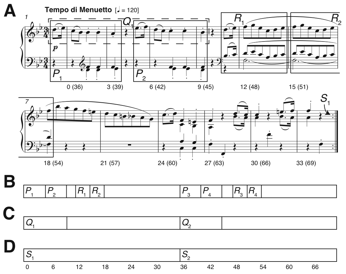
Existing approaches to music structure analysis in MIR tend to focus on segmentation (e.g., Weiss & Bello, 2010). The contribution of this task is to afford access to the note content itself (please see the example in Fig. 1A), requiring algorithms to do more than label time windows (e.g., the segmentations in Figs. 1B-D). For instance, a discovery algorithm applied to the piece in Fig. 1A should return a pattern corresponding to the note content of Failed to parse (MathML with SVG or PNG fallback (recommended for modern browsers and accessibility tools): Invalid response ("Math extension cannot connect to Restbase.") from server "https://wikimedia.org/api/rest_v1/":): {\displaystyle P_1} and Failed to parse (MathML with SVG or PNG fallback (recommended for modern browsers and accessibility tools): Invalid response ("Math extension cannot connect to Restbase.") from server "https://wikimedia.org/api/rest_v1/":): {\displaystyle P_2} , as well as a pattern corresponding to the note content of Failed to parse (MathML with SVG or PNG fallback (recommended for modern browsers and accessibility tools): Invalid response ("Math extension cannot connect to Restbase.") from server "https://wikimedia.org/api/rest_v1/":): {\displaystyle Q_1} . This is because Failed to parse (MathML with SVG or PNG fallback (recommended for modern browsers and accessibility tools): Invalid response ("Math extension cannot connect to Restbase.") from server "https://wikimedia.org/api/rest_v1/":): {\displaystyle Q_1} occurs again independently of the accompaniment in bars 19-22 (not shown here). The ground truth also contains nested patterns, such as Failed to parse (MathML with SVG or PNG fallback (recommended for modern browsers and accessibility tools): Invalid response ("Math extension cannot connect to Restbase.") from server "https://wikimedia.org/api/rest_v1/":): {\displaystyle P_1} in Fig. 1A being a subset of the sectional repetition Failed to parse (MathML with SVG or PNG fallback (recommended for modern browsers and accessibility tools): Invalid response ("Math extension cannot connect to Restbase.") from server "https://wikimedia.org/api/rest_v1/":): {\displaystyle S_1} , reflecting the often-hierarchical nature of musical repetition. While we recognise the appealing simplicity of linear segmentation, in the Discovery of Repeated Themes & Sections task we are demanding analysis at a greater level of detail, and have built a ground truth that contains overlapping and nested patterns.
Figure 1. Pattern discovery v segmentation. (A) Bars 1-12 of Mozart’s Piano Sonata in E-flat major K282 mvt.2, showing some ground-truth themes and repeated sections; (B-D) Three linear segmentations. Numbers below the staff in Fig. 1A and below the segmentation in Fig. 1D indicate crotchet beats, from zero for bar 1 beat 1.
For a more detailed introduction to the task, please see 2015:Discovery_of_Repeated_Themes_&_Sections.
Ground Truth and Algorithms
The ground truth, called the Johannes Kepler University Patterns Test Database (JKUPTD-Aug2013), is based on motifs and themes in Barlow and Morgenstern (1953), Schoenberg (1967), and Bruhn (1993). Repeated sections are based on those marked by the composer. These annotations are supplemented with some of our own where necessary. A Development Database (JKUPDD-Aug2013) enabled participants to try out their algorithms. For each piece in the Development and Test Databases, symbolic and synthesised audio versions are crossed with monophonic and polyphonic versions, giving four versions of the task in total: symPoly, symMono, audPoly, and audMono. There were no submissions to the symPoly category this year, so three versions of the task ran. Submitted algorithms are shown in Table 1.
| Sub code | Submission name | Abstract | Contributors |
|---|---|---|---|
| Task Version | symMono | ||
| PLM1 | SYMCHM | Matevz Pesek, Ales Leonardis, Matija Marolt | |
| OL1'14 | PatMinr | Olivier Lartillot | |
| VM2'14 | VM2 | Gissel Velarde, David Meredith | |
| Task Version | audMono | ||
| WHD1 | VMO Motif Discovery | Cheng-i Wang, Jennifer Hsu, Shlomo Dubnov | |
| WDH1 | VMO Motif Discovery FML | Cheng-i Wang, Jennifer Hsu, Shlomo Dubnov | |
| NF1'14 | MotivesExtractor | Oriol Nieto, Morwaread Farbood | |
| Task Version | audPoly | ||
| WHD1 | VMO Motif Discovery | Cheng-i Wang, Jennifer Hsu, Shlomo Dubnov | |
| WDH1 | VMO Motif Discovery FML | Cheng-i Wang, Jennifer Hsu, Shlomo Dubnov | |
| NF1'14 | MotivesExtractor | Oriol Nieto, Morwaread Farbood |
Table 1. Algorithms submitted to DRTS. Strong-performing algorithms from 2014 (submission codes ending '14) are included for the sake of comparisons.
Results in Brief
(For mathematical definitions of the various metrics, please see 2015:Discovery_of_Repeated_Themes_&_Sections#Evaluation_Procedure.)
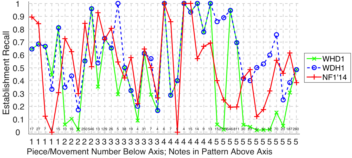
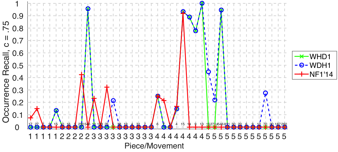
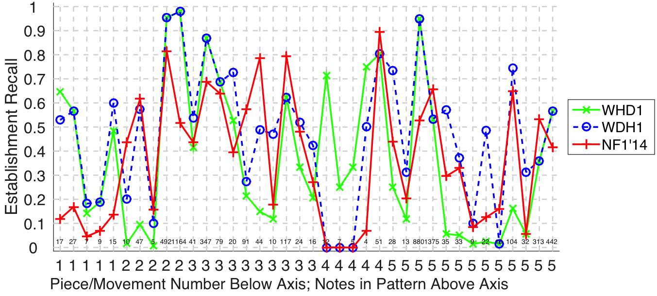
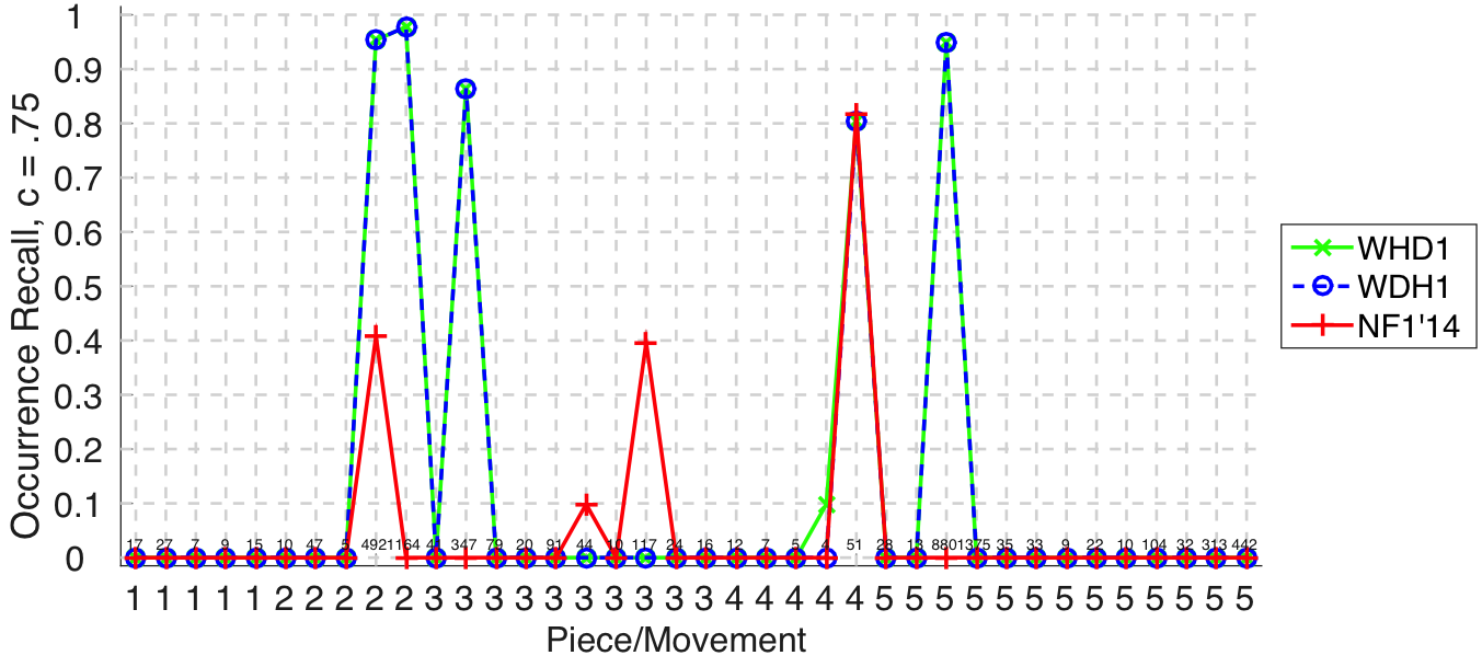
Wang, Hsu, and Dubnov (2015) submitted a motif discovery system based on a Variable Markov Oracle to audMono and audPoly versions of the task. On the audMono task this algorithm, WHD1, was not significantly different to NF1 according to Friedman's test (Failed to parse (MathML with SVG or PNG fallback (recommended for modern browsers and accessibility tools): Invalid response ("Math extension cannot connect to Restbase.") from server "https://wikimedia.org/api/rest_v1/":): {\displaystyle \chi^2(1) = .23,\ p = .631} ) at discovering at least one occurrence of each ground truth pattern (Fig. 14). Similarly, WHD1 was not significantly different to NF1 according to Friedman's test (Failed to parse (MathML with SVG or PNG fallback (recommended for modern browsers and accessibility tools): Invalid response ("Math extension cannot connect to Restbase.") from server "https://wikimedia.org/api/rest_v1/":): {\displaystyle \chi^2(1) = .89,\ p = .346} ) at discovering all occurrences of a given ground truth pattern (Fig. 15). These results suggest that WHD1 is on a par with state-of-the-art performance on the audMono task. Results for the audPoly task were similar, and WHD1 was significantly better than previous state-of-the-art performance (Failed to parse (MathML with SVG or PNG fallback (recommended for modern browsers and accessibility tools): Invalid response ("Math extension cannot connect to Restbase.") from server "https://wikimedia.org/api/rest_v1/":): {\displaystyle \chi^2(1) = 6.43,\ p =< .05} ) with regards discovering at least one occurrence of each ground truth pattern (Fig. ??).
Pesek, Leonardis, and Marolt (2015) submitted.
Nieto and Farbood (2014a) submitted to all four versions of the task (symbolic-monophonic, symbolic-polyphonic, audio-monophonic, audio-polyphonic), as they did last year (Nieto and Farbood, 2013). On the audio-monophonic version of the task, their NF1 algorithm’s Failed to parse (MathML with SVG or PNG fallback (recommended for modern browsers and accessibility tools): Invalid response ("Math extension cannot connect to Restbase.") from server "https://wikimedia.org/api/rest_v1/":): {\displaystyle F_1} scores were up by an average of .14 (establishing at least one occurrence of each ground truth pattern) and .11 (retrieving all occurrences of a discovered ground truth pattern) compared to last year (see Figs. 30 and 33). There were slighter increases in the audio-polyphonic version of the task. Their work on extracting repetitive structure remains at the forefront of research attempting to cross the audio-symbolic divide (Nieto & Farbood, 2014b; Collins et al., 2014).
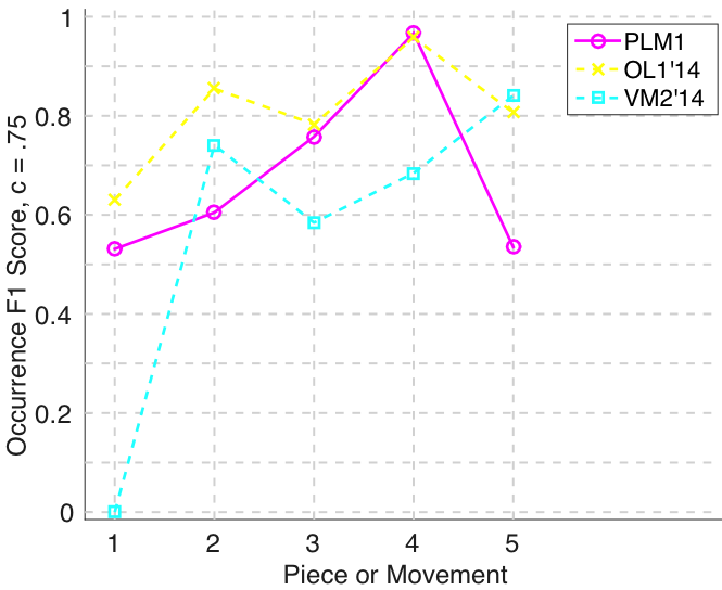
Lartillot (2014a, 2014b) submitted an incremental pattern mining algorithm to the symbolic-monophonic version of the task this year. The musical dimensions represented (e.g., chromatic pitch, diatonic pitch) are able to vary throughout the course of a pattern occurrence. The ability to vary representation within an occurrence should mean that Lartillot’s OL1 algorithm is well prepared for retrieving both exact and inexact occurrences of motifs and themes. This does seem to be the case, with OL1 the strongest performer on the occurrence Failed to parse (MathML with SVG or PNG fallback (recommended for modern browsers and accessibility tools): Invalid response ("Math extension cannot connect to Restbase.") from server "https://wikimedia.org/api/rest_v1/":): {\displaystyle F_1} metric (Fig. 9).
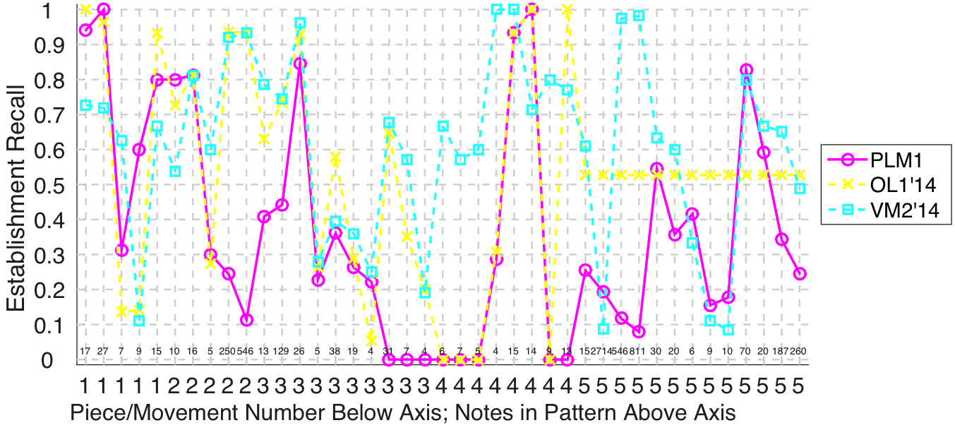
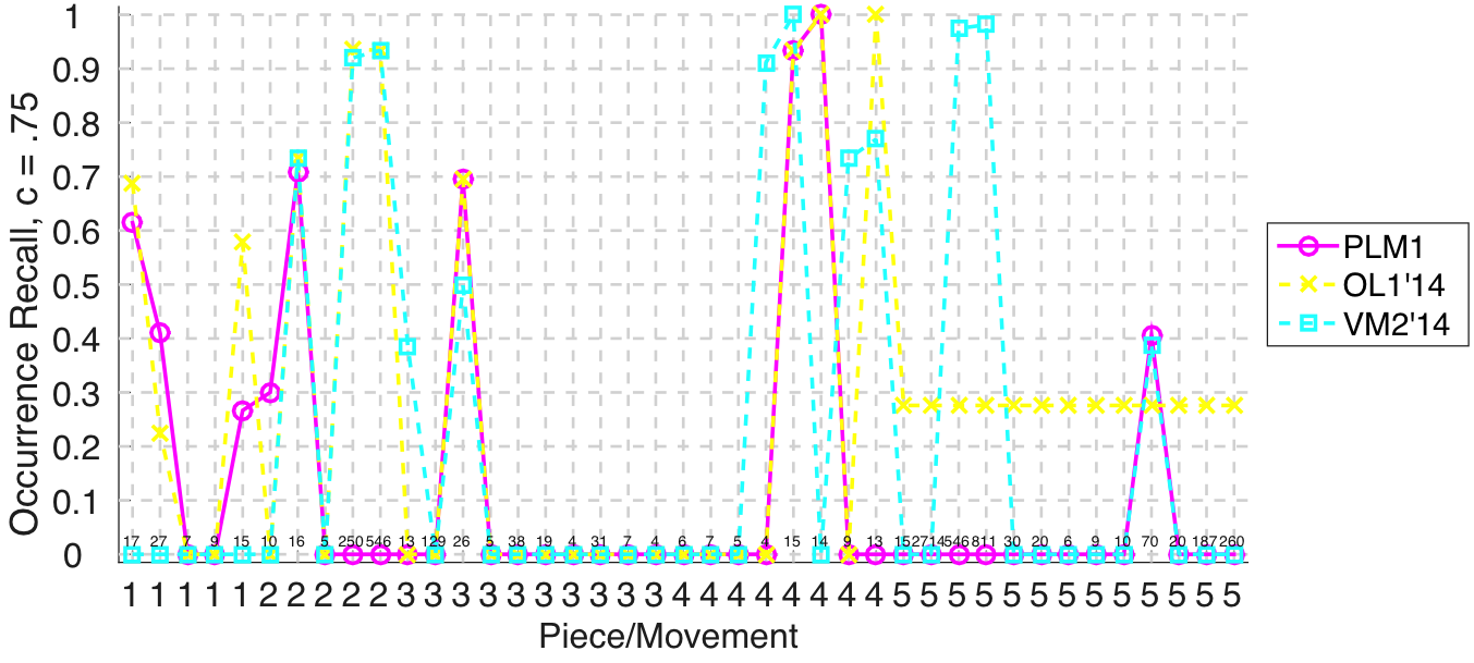
Velarde and Meredith (2014) submitted a wavelet-based method to the symbolic-monophonic version of the task this year. This algorithm, VM1, tested significantly stronger according to Friedman's test than NF1 (Failed to parse (MathML with SVG or PNG fallback (recommended for modern browsers and accessibility tools): Invalid response ("Math extension cannot connect to Restbase.") from server "https://wikimedia.org/api/rest_v1/":): {\displaystyle \chi^2(1) = 25,\ p < .001} , Bonferroni-corrected) and OL1 (Failed to parse (MathML with SVG or PNG fallback (recommended for modern browsers and accessibility tools): Invalid response ("Math extension cannot connect to Restbase.") from server "https://wikimedia.org/api/rest_v1/":): {\displaystyle \chi^2(1) = 17.86,\ p < .001} , Bonferroni-corrected) at discovering at least one occurrence of each ground truth pattern (Fig. 2). While VM1 also seems to find lots of occurrences of each ground truth pattern (with high occurrence recall in Fig. 7, and in Fig. 3 on a per-pattern basis), it may also find quite a few false-positive occurrences (with lower occurrence precision in Fig. 8). (To avoid a bias toward the more numerous submissions of Velarde and Meredith (2014), VM1 was preselected for comparison with Nieto and Farbood's (2014a) and Lartillot's (2014a) submissions, based on performance for the Development Database.)
Discussion
Last year it was observed that the discovery of repeated sections was addressed well by the submissions, but that the discovery of themes and motifs required more attention in future iterations of this task. There has been some improvement in this regard: VM1 scores better on establishment recall (Fig. 2) than last year's algorithms, for pattern occurrences in pieces 1-3 that contain 7, 9, 5, and 4 notes.
It was pleasing to see Nieto and Farbood’s (2014a) results improve by 10-15% compared with last year on the audio-monophonic version of the task. This improvement underlines the importance of the Discovery of Repeated Themes and Sections task in helping researchers to push the boundaries of music informatics research.
It was exciting to see more participants than last year converge on one particular task version, from which Lartillot (2014a) emerged with the strongest results for retrieving exact and inexact occurrences of already-discovered patterns, and Velarde and Meredith (2014) emerged with an impressively strong algorithm for discovering at least one occurrence of each ground truth pattern.
Next year it would be great to see yet more researchers with relevant algorithms engaging in the task (Conklin & Bergeron, 2008; Giraud et al., in press; Müller & Jiang, 2012; Peters & Deruty, 2009). I have already made (and am happy to make) amendments/additions to the databases in order to encourage participation. A renewed effort to tackle the polyphonic versions of this task would also be most welcome, as these are inherently harder but perhaps more interesting for that reason. These polyphonic scenarios have more immediate applications in the support of other MIR tasks (e.g., beat tracking and/or expressive rendering might be improved by knowledge of motif/theme/section locations), so it would also be great to see some research developing in this direction too.
Tom Collins, Leicester, 2014
Results in Detail
symMono
(Submission OL1 did not complete on piece 5. The task captain took the decision to assign the mean of the evaluation metrics for OL1 calculated across the remaining pieces.)
Figure 2. Establishment recall on a per-pattern basis. Establishment recall answers the following question. On average, how similar is the most similar algorithm-output pattern to a ground-truth pattern prototype?
Figure 3. Occurrence recall on a per-pattern basis. Occurrence recall answers the following question. On average, how similar is the most similar set of algorithm-output pattern occurrences to a discovered ground-truth occurrence set?
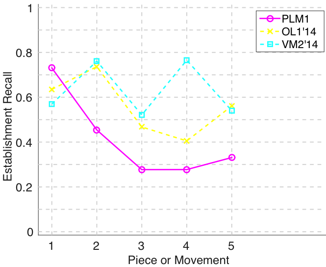
Figure 4. Establishment recall averaged over each piece/movement. Establishment recall answers the following question. On average, how similar is the most similar algorithm-output pattern to a ground-truth pattern prototype?
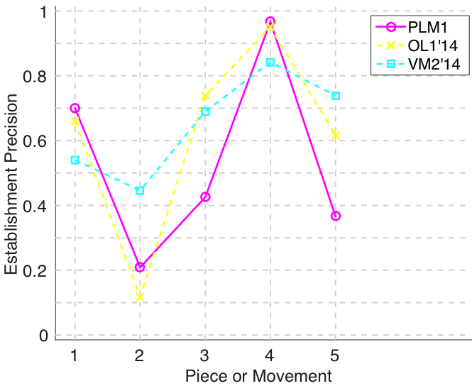
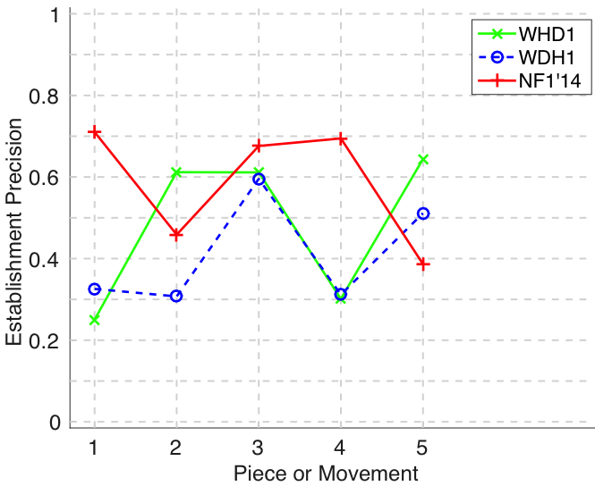
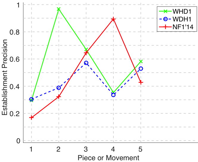
Figure 5. Establishment precision averaged over each piece/movement. Establishment precision answers the following question. On average, how similar is the most similar ground-truth pattern prototype to an algorithm-output pattern?
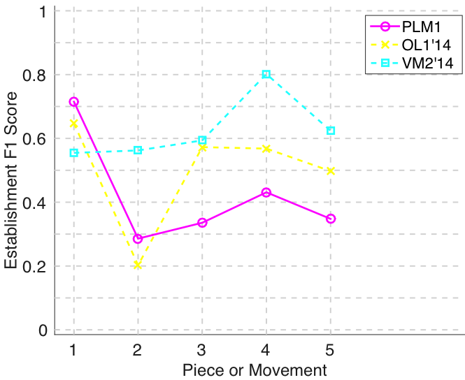
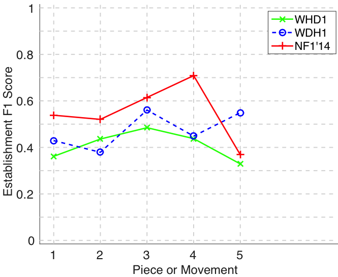
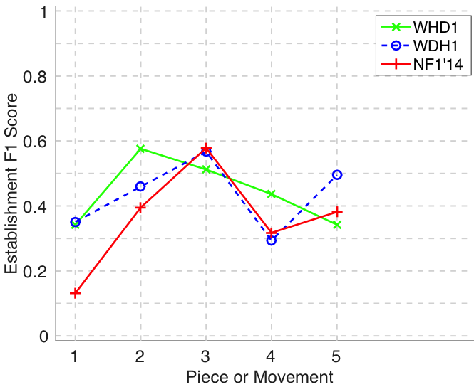
Figure 6. Establishment F1 averaged over each piece/movement. Establishment F1 is an average of establishment precision and establishment recall.
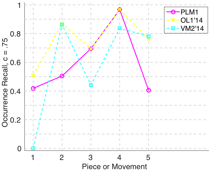
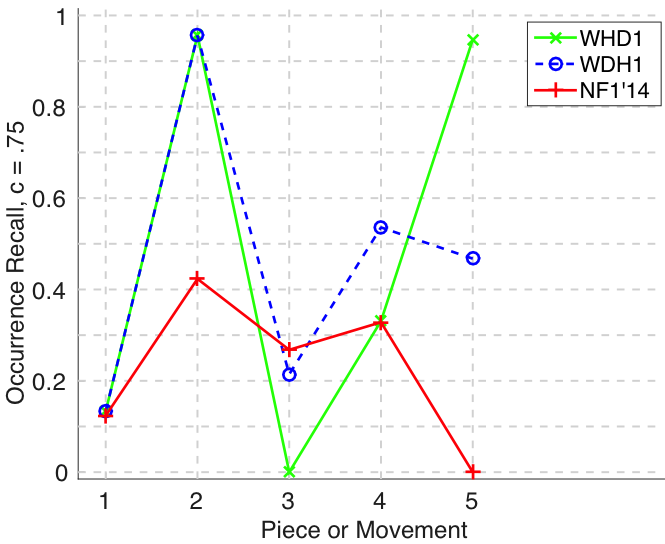
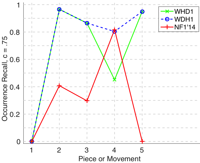
Figure 7. Occurrence recall (Failed to parse (MathML with SVG or PNG fallback (recommended for modern browsers and accessibility tools): Invalid response ("Math extension cannot connect to Restbase.") from server "https://wikimedia.org/api/rest_v1/":): {\displaystyle c = .75} ) averaged over each piece/movement. Occurrence recall answers the following question. On average, how similar is the most similar set of algorithm-output pattern occurrences to a discovered ground-truth occurrence set?
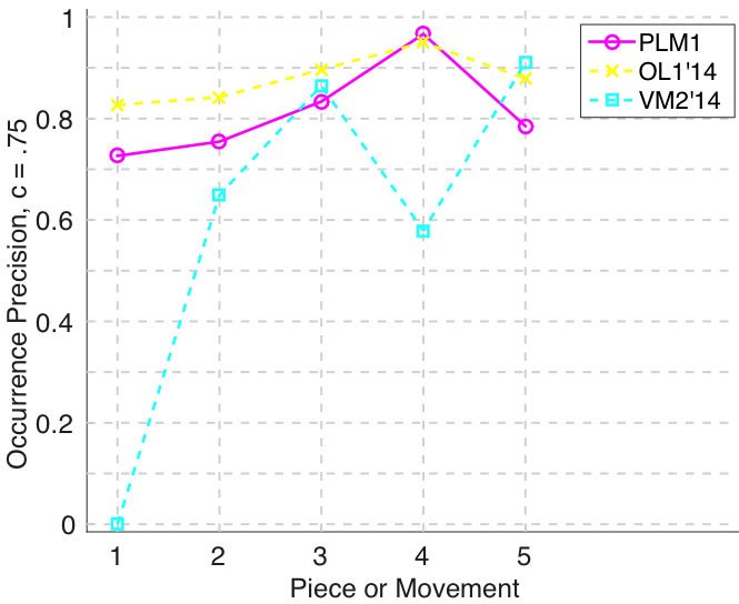
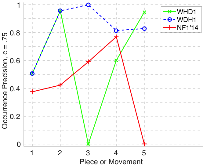
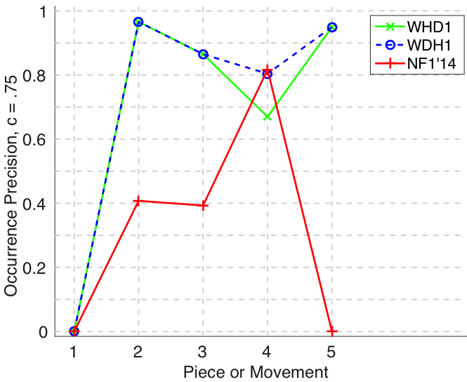
Figure 8. Occurrence precision (Failed to parse (MathML with SVG or PNG fallback (recommended for modern browsers and accessibility tools): Invalid response ("Math extension cannot connect to Restbase.") from server "https://wikimedia.org/api/rest_v1/":): {\displaystyle c = .75} ) averaged over each piece/movement. Occurrence precision answers the following question. On average, how similar is the most similar discovered ground-truth occurrence set to a set of algorithm-output pattern occurrences?
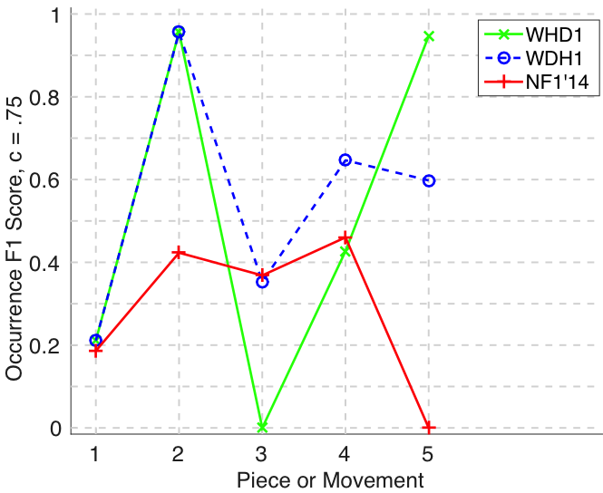
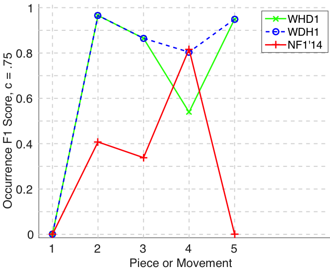
Figure 9. Occurrence F1 (Failed to parse (MathML with SVG or PNG fallback (recommended for modern browsers and accessibility tools): Invalid response ("Math extension cannot connect to Restbase.") from server "https://wikimedia.org/api/rest_v1/":): {\displaystyle c = .75} ) averaged over each piece/movement. Occurrence F1 is an average of occurrence precision and occurrence recall.
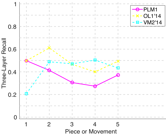
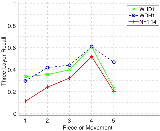
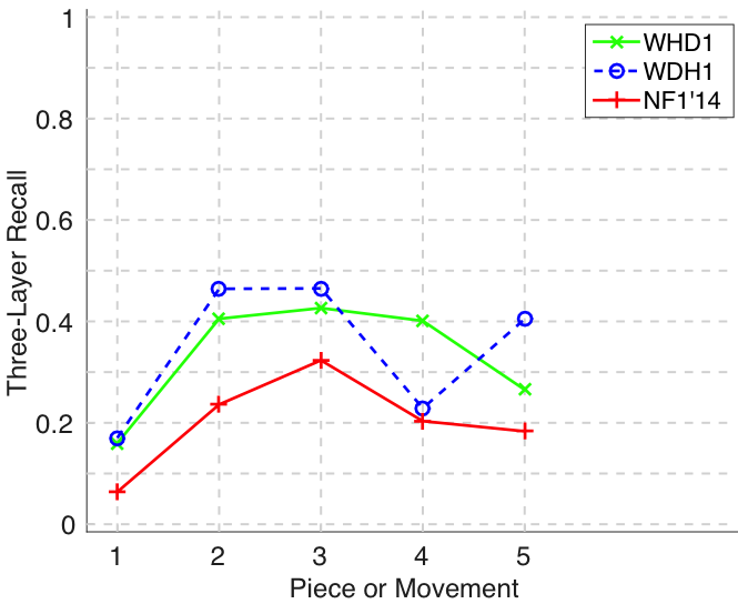
Figure 10. Three-layer recall averaged over each piece/movement. Rather than using Failed to parse (MathML with SVG or PNG fallback (recommended for modern browsers and accessibility tools): Invalid response ("Math extension cannot connect to Restbase.") from server "https://wikimedia.org/api/rest_v1/":): {\displaystyle |P \cap Q|/\max\{|P|, |Q|\}} as a similarity measure (which is the default for establishment recall), three-layer recall uses Failed to parse (MathML with SVG or PNG fallback (recommended for modern browsers and accessibility tools): Invalid response ("Math extension cannot connect to Restbase.") from server "https://wikimedia.org/api/rest_v1/":): {\displaystyle 2|P \cap Q|/(|P| + |Q|)} , which is a kind of F1 measure.
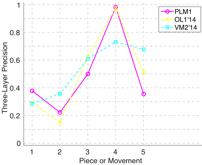
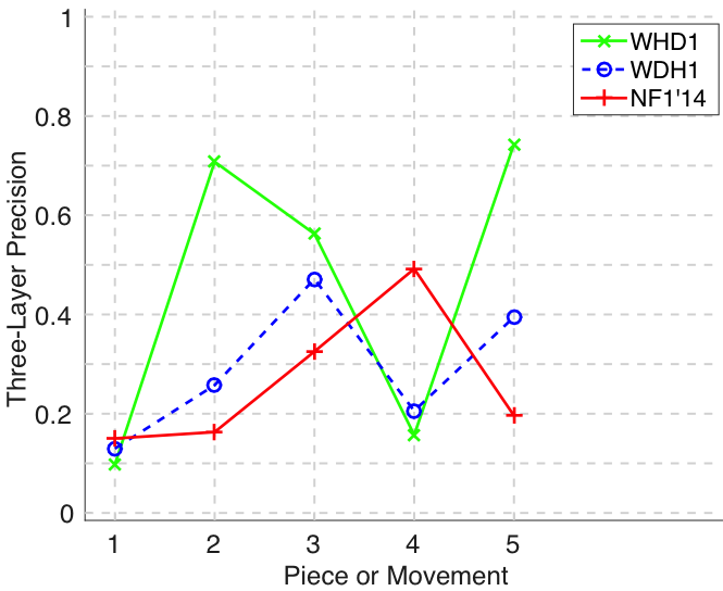
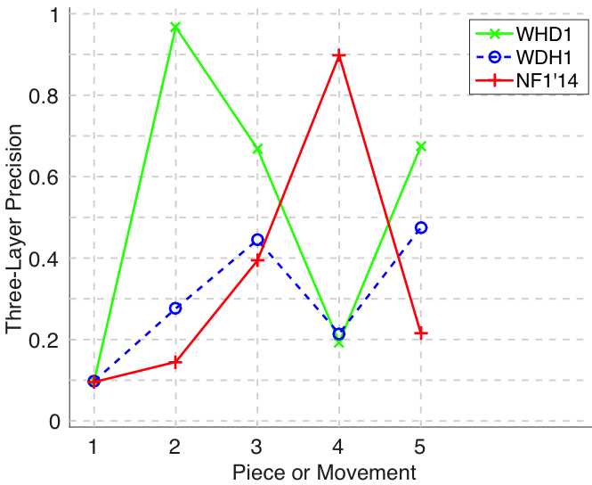
Figure 11. Three-layer precision averaged over each piece/movement. Rather than using Failed to parse (MathML with SVG or PNG fallback (recommended for modern browsers and accessibility tools): Invalid response ("Math extension cannot connect to Restbase.") from server "https://wikimedia.org/api/rest_v1/":): {\displaystyle |P \cap Q|/\max\{|P|, |Q|\}} as a similarity measure (which is the default for establishment precision), three-layer precision uses Failed to parse (MathML with SVG or PNG fallback (recommended for modern browsers and accessibility tools): Invalid response ("Math extension cannot connect to Restbase.") from server "https://wikimedia.org/api/rest_v1/":): {\displaystyle 2|P \cap Q|/(|P| + |Q|)} , which is a kind of F1 measure.
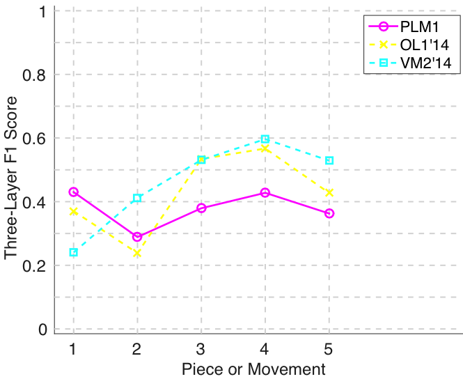
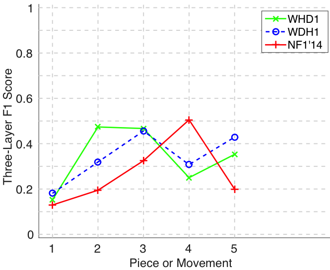
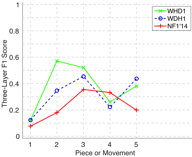
Figure 12. Three-layer F1 (TLF) averaged over each piece/movement. TLF is an average of three-layer precision and three-layer recall.
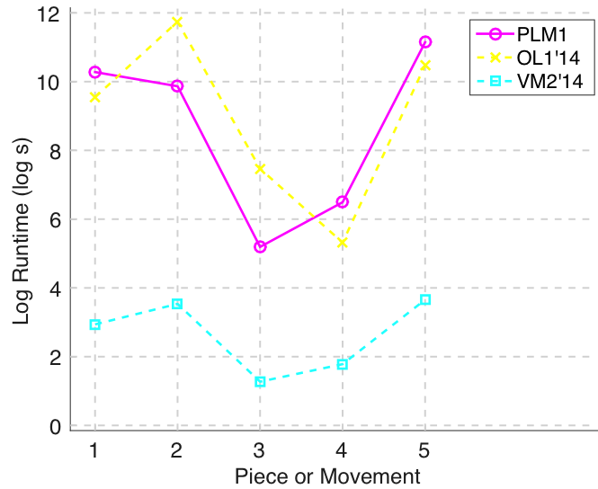
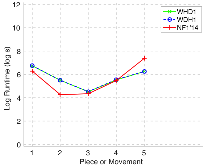
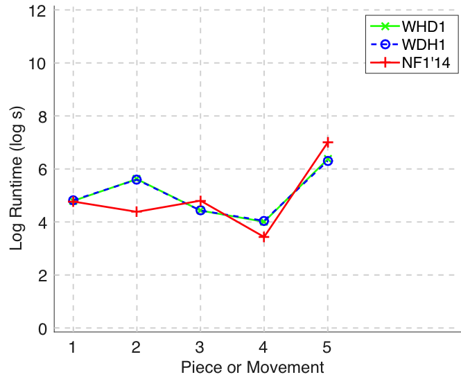
Figure 13. Log runtime of the algorithm for each piece/movement.
audMono
Figure 14. Establishment recall on a per-pattern basis. Establishment recall answers the following question. On average, how similar is the most similar algorithm-output pattern to a ground-truth pattern prototype?
Figure 15. Occurrence recall on a per-pattern basis. Occurrence recall answers the following question. On average, how similar is the most similar set of algorithm-output pattern occurrences to a discovered ground-truth occurrence set?
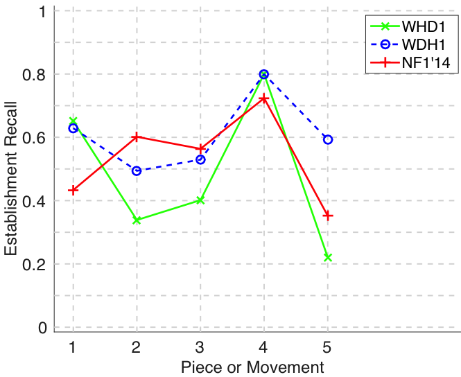
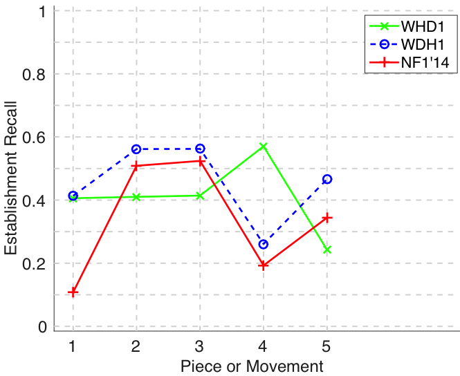
Figure 16. Establishment recall averaged over each piece/movement. Establishment recall answers the following question. On average, how similar is the most similar algorithm-output pattern to a ground-truth pattern prototype?
Figure 17. Establishment precision averaged over each piece/movement. Establishment precision answers the following question. On average, how similar is the most similar ground-truth pattern prototype to an algorithm-output pattern?
Figure 18. Establishment F1 averaged over each piece/movement. Establishment F1 is an average of establishment precision and establishment recall.
Figure 19. Occurrence recall (Failed to parse (MathML with SVG or PNG fallback (recommended for modern browsers and accessibility tools): Invalid response ("Math extension cannot connect to Restbase.") from server "https://wikimedia.org/api/rest_v1/":): {\displaystyle c = .75} ) averaged over each piece/movement. Occurrence recall answers the following question. On average, how similar is the most similar set of algorithm-output pattern occurrences to a discovered ground-truth occurrence set?
Figure 20. Occurrence precision (Failed to parse (MathML with SVG or PNG fallback (recommended for modern browsers and accessibility tools): Invalid response ("Math extension cannot connect to Restbase.") from server "https://wikimedia.org/api/rest_v1/":): {\displaystyle c = .75} ) averaged over each piece/movement. Occurrence precision answers the following question. On average, how similar is the most similar discovered ground-truth occurrence set to a set of algorithm-output pattern occurrences?
Figure 21. Occurrence F1 (Failed to parse (MathML with SVG or PNG fallback (recommended for modern browsers and accessibility tools): Invalid response ("Math extension cannot connect to Restbase.") from server "https://wikimedia.org/api/rest_v1/":): {\displaystyle c = .75} ) averaged over each piece/movement. Occurrence F1 is an average of occurrence precision and occurrence recall.
Figure 22. Three-layer recall averaged over each piece/movement. Rather than using Failed to parse (MathML with SVG or PNG fallback (recommended for modern browsers and accessibility tools): Invalid response ("Math extension cannot connect to Restbase.") from server "https://wikimedia.org/api/rest_v1/":): {\displaystyle |P \cap Q|/\max\{|P|, |Q|\}} as a similarity measure (which is the default for establishment recall), three-layer recall uses Failed to parse (MathML with SVG or PNG fallback (recommended for modern browsers and accessibility tools): Invalid response ("Math extension cannot connect to Restbase.") from server "https://wikimedia.org/api/rest_v1/":): {\displaystyle 2|P \cap Q|/(|P| + |Q|)} , which is a kind of F1 measure.
Figure 23. Three-layer precision averaged over each piece/movement. Rather than using Failed to parse (MathML with SVG or PNG fallback (recommended for modern browsers and accessibility tools): Invalid response ("Math extension cannot connect to Restbase.") from server "https://wikimedia.org/api/rest_v1/":): {\displaystyle |P \cap Q|/\max\{|P|, |Q|\}} as a similarity measure (which is the default for establishment precision), three-layer precision uses Failed to parse (MathML with SVG or PNG fallback (recommended for modern browsers and accessibility tools): Invalid response ("Math extension cannot connect to Restbase.") from server "https://wikimedia.org/api/rest_v1/":): {\displaystyle 2|P \cap Q|/(|P| + |Q|)} , which is a kind of F1 measure.
Figure 24. Three-layer F1 (TLF) averaged over each piece/movement. TLF is an average of three-layer precision and three-layer recall.
Figure 25. Log runtime of the algorithm for each piece/movement.
audPoly
Figure 38. Establishment recall on a per-pattern basis. Establishment recall answers the following question. On average, how similar is the most similar algorithm-output pattern to a ground-truth pattern prototype?
Figure 39. Occurrence recall on a per-pattern basis. Occurrence recall answers the following question. On average, how similar is the most similar set of algorithm-output pattern occurrences to a discovered ground-truth occurrence set?
Figure 40. Establishment recall averaged over each piece/movement. Establishment recall answers the following question. On average, how similar is the most similar algorithm-output pattern to a ground-truth pattern prototype?
Figure 41. Establishment precision averaged over each piece/movement. Establishment precision answers the following question. On average, how similar is the most similar ground-truth pattern prototype to an algorithm-output pattern?
Figure 42. Establishment F1 averaged over each piece/movement. Establishment F1 is an average of establishment precision and establishment recall.
Figure 43. Occurrence recall (Failed to parse (MathML with SVG or PNG fallback (recommended for modern browsers and accessibility tools): Invalid response ("Math extension cannot connect to Restbase.") from server "https://wikimedia.org/api/rest_v1/":): {\displaystyle c = .75} ) averaged over each piece/movement. Occurrence recall answers the following question. On average, how similar is the most similar set of algorithm-output pattern occurrences to a discovered ground-truth occurrence set?
Figure 44. Occurrence precision (Failed to parse (MathML with SVG or PNG fallback (recommended for modern browsers and accessibility tools): Invalid response ("Math extension cannot connect to Restbase.") from server "https://wikimedia.org/api/rest_v1/":): {\displaystyle c = .75} ) averaged over each piece/movement. Occurrence precision answers the following question. On average, how similar is the most similar discovered ground-truth occurrence set to a set of algorithm-output pattern occurrences?
Figure 45. Occurrence F1 (Failed to parse (MathML with SVG or PNG fallback (recommended for modern browsers and accessibility tools): Invalid response ("Math extension cannot connect to Restbase.") from server "https://wikimedia.org/api/rest_v1/":): {\displaystyle c = .75} ) averaged over each piece/movement. Occurrence F1 is an average of occurrence precision and occurrence recall.
Figure 46. Three-layer recall averaged over each piece/movement. Rather than using Failed to parse (MathML with SVG or PNG fallback (recommended for modern browsers and accessibility tools): Invalid response ("Math extension cannot connect to Restbase.") from server "https://wikimedia.org/api/rest_v1/":): {\displaystyle |P \cap Q|/\max\{|P|, |Q|\}} as a similarity measure (which is the default for establishment recall), three-layer recall uses Failed to parse (MathML with SVG or PNG fallback (recommended for modern browsers and accessibility tools): Invalid response ("Math extension cannot connect to Restbase.") from server "https://wikimedia.org/api/rest_v1/":): {\displaystyle 2|P \cap Q|/(|P| + |Q|)} , which is a kind of F1 measure.
Figure 47. Three-layer precision averaged over each piece/movement. Rather than using Failed to parse (MathML with SVG or PNG fallback (recommended for modern browsers and accessibility tools): Invalid response ("Math extension cannot connect to Restbase.") from server "https://wikimedia.org/api/rest_v1/":): {\displaystyle |P \cap Q|/\max\{|P|, |Q|\}} as a similarity measure (which is the default for establishment precision), three-layer precision uses Failed to parse (MathML with SVG or PNG fallback (recommended for modern browsers and accessibility tools): Invalid response ("Math extension cannot connect to Restbase.") from server "https://wikimedia.org/api/rest_v1/":): {\displaystyle 2|P \cap Q|/(|P| + |Q|)} , which is a kind of F1 measure.
Figure 48. Three-layer F1 (TLF) averaged over each piece/movement. TLF is an average of three-layer precision and three-layer recall.
Figure 49. Log runtime of the algorithm for each piece/movement.
Tabular Versions of Plots
symMono
| AlgIdx | AlgStub | Piece | n_P | n_Q | P_est | R_est | F1_est | P_occ(c=.75) | R_occ(c=.75) | F_1occ(c=.75) | P_3 | R_3 | TLF_1 | runtime | FRT | FFTP_est | FFP | P_occ(c=.5) | R_occ(c=.5) | F_1occ(c=.5) | P | R | F_1 |
|---|---|---|---|---|---|---|---|---|---|---|---|---|---|---|---|---|---|---|---|---|---|---|---|
| 1 | PLM1 | piece1 | 5 | 18.000 | 0.700 | 0.731 | 0.715 | 0.726 | 0.419 | 0.531 | 0.378 | 0.499 | 0.430 | 29100.000 | 0.000 | 0.480 | 0.294 | 0.579 | 0.433 | 0.495 | 0.000 | 0.000 | 0.000 |
| 1 | PLM1 | piece2 | 5 | 31.000 | 0.209 | 0.454 | 0.286 | 0.755 | 0.505 | 0.605 | 0.222 | 0.413 | 0.289 | 19260.000 | 0.000 | 0.174 | 0.177 | 0.670 | 0.573 | 0.617 | 0.032 | 0.200 | 0.056 |
| 1 | PLM1 | piece3 | 10.000 | 8 | 0.426 | 0.277 | 0.336 | 0.834 | 0.695 | 0.758 | 0.501 | 0.305 | 0.379 | 180.000 | 0.000 | 0.242 | 0.505 | 0.834 | 0.695 | 0.758 | 0.000 | 0.000 | 0.000 |
| 1 | PLM1 | piece4 | 8 | 2 | 0.967 | 0.277 | 0.431 | 0.967 | 0.967 | 0.967 | 0.983 | 0.273 | 0.428 | 660.000 | 0.000 | 0.277 | 0.983 | 0.967 | 0.967 | 0.967 | 0.500 | 0.125 | 0.200 |
| 1 | PLM1 | piece5 | 13.000 | 35.000 | 0.366 | 0.331 | 0.348 | 0.785 | 0.406 | 0.535 | 0.354 | 0.372 | 0.363 | 69240.000 | 0.000 | 0.103 | 0.226 | 0.617 | 0.456 | 0.525 | 0.000 | 0.000 | 0.000 |
| 2 | OL1_14 | piece1 | 5 | 114.000 | 0.660 | 0.635 | 0.647 | 0.827 | 0.509 | 0.630 | 0.295 | 0.498 | 0.370 | 14013.284 | 0.000 | 0.368 | 0.389 | 0.723 | 0.559 | 0.630 | 0.009 | 0.200 | 0.017 |
| 2 | OL1_14 | piece2 | 5 | 98.000 | 0.117 | 0.737 | 0.202 | 0.842 | 0.868 | 0.855 | 0.148 | 0.611 | 0.238 | 126065.856 | 0.000 | 0.277 | 0.440 | 0.750 | 0.709 | 0.729 | 0.020 | 0.400 | 0.039 |
| 2 | OL1_14 | piece3 | 10.000 | 9 | 0.739 | 0.467 | 0.573 | 0.897 | 0.695 | 0.783 | 0.625 | 0.466 | 0.534 | 1751.959 | 0.000 | 0.348 | 0.622 | 0.728 | 0.608 | 0.663 | 0.111 | 0.100 | 0.105 |
| 2 | OL1_14 | piece4 | 8 | 4 | 0.950 | 0.405 | 0.568 | 0.950 | 0.967 | 0.958 | 0.974 | 0.400 | 0.567 | 204.197 | 0.000 | 0.405 | 0.974 | 0.950 | 0.967 | 0.958 | 0.500 | 0.250 | 0.333 |
| 2 | OL1_14 | piece5 | 13.000 | 56.250 | 0.617 | 0.561 | 0.498 | 0.879 | 0.760 | 0.807 | 0.510 | 0.494 | 0.427 | 35508.820 | 0.000 | 0.350 | 0.606 | 0.788 | 0.711 | 0.745 | 0.160 | 0.237 | 0.124 |
| 3 | VM2_14 | piece1 | 5 | 5 | 0.540 | 0.570 | 0.555 | 0.000 | 0.000 | 0.000 | 0.286 | 0.207 | 0.240 | 18.906 | 0.000 | 0.570 | 0.286 | 0.291 | 0.490 | 0.365 | 0.000 | 0.000 | 0.000 |
| 3 | VM2_14 | piece2 | 5 | 7 | 0.446 | 0.761 | 0.562 | 0.649 | 0.863 | 0.741 | 0.357 | 0.488 | 0.413 | 34.308 | 0.000 | 0.419 | 0.128 | 0.427 | 0.630 | 0.509 | 0.143 | 0.200 | 0.167 |
| 3 | VM2_14 | piece3 | 10.000 | 7 | 0.690 | 0.521 | 0.594 | 0.865 | 0.441 | 0.584 | 0.609 | 0.471 | 0.531 | 3.570 | 0.000 | 0.393 | 0.541 | 0.662 | 0.561 | 0.607 | 0.000 | 0.000 | 0.000 |
| 3 | VM2_14 | piece4 | 8 | 6 | 0.842 | 0.765 | 0.802 | 0.579 | 0.837 | 0.684 | 0.732 | 0.504 | 0.597 | 5.942 | 0.000 | 0.721 | 0.711 | 0.410 | 0.732 | 0.525 | 0.167 | 0.125 | 0.143 |
| 3 | VM2_14 | piece5 | 13.000 | 7 | 0.739 | 0.540 | 0.624 | 0.910 | 0.781 | 0.841 | 0.677 | 0.434 | 0.529 | 38.698 | 0.000 | 0.420 | 0.554 | 0.517 | 0.636 | 0.570 | 0.000 | 0.000 | 0.000 |
Table 2. Tabular version of Figures 4-13.
| AlgIdx | AlgStub | Piece | n_P | R_est | R_occ(c=.75) | R_occ(c=.5) | ||||||
|---|---|---|---|---|---|---|---|---|---|---|---|---|
| 1 | PLM1 | piece1 | 5 | |||||||||
| 0.941 | 1.000 | 0.312 | 0.600 | 0.800 | ||||||||
| 0.614 | 0.410 | 0.000 | 0.000 | 0.267 | ||||||||
| 0.614 | 0.410 | 0.000 | 0.000 | 0.267 | ||||||||
| 1 | PLM1 | piece2 | 5 | |||||||||
| 0.800 | 0.812 | 0.300 | 0.244 | 0.114 | ||||||||
| 0.300 | 0.709 | 0.000 | 0.000 | 0.000 | ||||||||
| 0.300 | 0.709 | 0.000 | 0.000 | 0.000 | ||||||||
| 1 | PLM1 | piece3 | 10.000 | |||||||||
| 0.409 | 0.442 | 0.846 | 0.227 | 0.361 | 0.263 | 0.222 | 0.000 | 0.000 | 0.000 | |||
| 0.00000 | 0.000 | 0.695 | 0.000 | 0.000 | 0.000 | 0.000 | 0.000 | 0.000 | 0.000 | |||
| 0.00000 | 0.000 | 0.695 | 0.000 | 0.000 | 0.000 | 0.000 | 0.000 | 0.000 | 0.000 | |||
| 1 | PLM1 | piece4 | 8 | |||||||||
| 0.00000 | 0.000 | 0.000 | 0.286 | 0.933 | 1.000 | 0.000 | 0.000 | |||||
| 0.00000 | 0.000 | 0.000 | 0.000 | 0.933 | 1.000 | 0.000 | 0.000 | |||||
| 0.00000 | 0.000 | 0.000 | 0.000 | 0.933 | 1.000 | 0.000 | 0.000 | |||||
| 1 | PLM1 | piece5 | 13.000 | |||||||||
| 0.255 | 0.193 | 0.117 | 0.079 | 0.545 | 0.357 | 0.417 | 0.155 | 0.177 | 0.829 | 0.591 | 0.342 | 0.246 |
| 0.00000 | 0.000 | 0.000 | 0.000 | 0.000 | 0.000 | 0.000 | 0.000 | 0.000 | 0.406 | 0.000 | 0.000 | 0.000 |
| 0.00000 | 0.000 | 0.000 | 0.000 | 0.000 | 0.000 | 0.000 | 0.000 | 0.000 | 0.406 | 0.000 | 0.000 | 0.000 |
| 2 | OL1_14 | piece1 | 5 | |||||||||
| 1.00000 | 0.964 | 0.137 | 0.140 | 0.933 | ||||||||
| 0.688 | 0.226 | 0.000 | 0.000 | 0.578 | ||||||||
| 0.688 | 0.226 | 0.000 | 0.000 | 0.578 | ||||||||
| 2 | OL1_14 | piece2 | 5 | |||||||||
| 0.727 | 0.812 | 0.273 | 0.936 | 0.934 | ||||||||
| 0.00000 | 0.734 | 0.000 | 0.936 | 0.934 | ||||||||
| 0.00000 | 0.734 | 0.000 | 0.936 | 0.934 | ||||||||
| 2 | OL1_14 | piece3 | 10.000 | |||||||||
| 0.632 | 0.735 | 0.929 | 0.263 | 0.579 | 0.289 | 0.053 | 0.645 | 0.350 | 0.200 | |||
| 0.00000 | 0.000 | 0.695 | 0.000 | 0.000 | 0.000 | 0.000 | 0.000 | 0.000 | 0.000 | |||
| 0.00000 | 0.000 | 0.695 | 0.000 | 0.000 | 0.000 | 0.000 | 0.000 | 0.000 | 0.000 | |||
| 2 | OL1_14 | piece4 | 8 | |||||||||
| 0.00000 | 0.000 | 0.000 | 0.308 | 0.933 | 1.000 | 0.000 | 1.000 | |||||
| 0.00000 | 0.000 | 0.000 | 0.000 | 0.933 | 1.000 | 0.000 | 1.000 | |||||
| 0.00000 | 0.000 | 0.000 | 0.000 | 0.933 | 1.000 | 0.000 | 1.000 | |||||
| 2 | OL1_14 | piece5 | 13.000 | |||||||||
| 0.528 | 0.528 | 0.528 | 0.528 | 0.528 | 0.528 | 0.528 | 0.528 | 0.528 | 0.528 | 0.528 | 0.528 | 0.528 |
| 0.276 | 0.276 | 0.276 | 0.276 | 0.276 | 0.276 | 0.276 | 0.276 | 0.276 | 0.276 | 0.276 | 0.276 | 0.276 |
| 0.276 | 0.276 | 0.276 | 0.276 | 0.276 | 0.276 | 0.276 | 0.276 | 0.276 | 0.276 | 0.276 | 0.276 | 0.276 |
| 3 | VM2_14 | piece1 | 5 | |||||||||
| 0.727 | 0.719 | 0.625 | 0.111 | 0.667 | ||||||||
| 0.00000 | 0.000 | 0.000 | 0.000 | 0.000 | ||||||||
| 0.00000 | 0.000 | 0.000 | 0.000 | 0.000 | ||||||||
| 3 | VM2_14 | piece2 | 5 | |||||||||
| 0.538 | 0.812 | 0.600 | 0.920 | 0.934 | ||||||||
| 0.00000 | 0.734 | 0.000 | 0.920 | 0.934 | ||||||||
| 0.00000 | 0.734 | 0.000 | 0.920 | 0.934 | ||||||||
| 3 | VM2_14 | piece3 | 10.000 | |||||||||
| 0.786 | 0.744 | 0.962 | 0.278 | 0.395 | 0.360 | 0.250 | 0.677 | 0.571 | 0.190 | |||
| 0.384 | 0.000 | 0.498 | 0.000 | 0.000 | 0.000 | 0.000 | 0.000 | 0.000 | 0.000 | |||
| 0.384 | 0.000 | 0.498 | 0.000 | 0.000 | 0.000 | 0.000 | 0.000 | 0.000 | 0.000 | |||
| 3 | VM2_14 | piece4 | 8 | |||||||||
| 0.667 | 0.571 | 0.600 | 1.000 | 1.000 | 0.714 | 0.800 | 0.769 | |||||
| 0.00000 | 0.000 | 0.000 | 0.911 | 1.000 | 0.000 | 0.733 | 0.769 | |||||
| 0.00000 | 0.000 | 0.000 | 0.911 | 1.000 | 0.000 | 0.733 | 0.769 | |||||
| 3 | VM2_14 | piece5 | 13.000 | |||||||||
| 0.609 | 0.087 | 0.974 | 0.982 | 0.633 | 0.600 | 0.333 | 0.111 | 0.084 | 0.800 | 0.667 | 0.652 | 0.488 |
| 0.00000 | 0.000 | 0.974 | 0.982 | 0.000 | 0.000 | 0.000 | 0.000 | 0.000 | 0.388 | 0.000 | 0.000 | 0.000 |
| 0.00000 | 0.000 | 0.974 | 0.982 | 0.000 | 0.000 | 0.000 | 0.000 | 0.000 | 0.388 | 0.000 | 0.000 | 0.000 |
Table 3. Tabular version of Figures 2 and 3.
audMono
| AlgIdx | AlgStub | Piece | n_P | n_Q | P_est | R_est | F1_est | P_occ(c=.75) | R_occ(c=.75) | F_1occ(c=.75) | P_3 | R_3 | TLF_1 | runtime | FRT | FFTP_est | FFP | P_occ(c=.5) | R_occ(c=.5) | F_1occ(c=.5) | P | R | F_1 |
|---|---|---|---|---|---|---|---|---|---|---|---|---|---|---|---|---|---|---|---|---|---|---|---|
| 1 | WHD1 | piece1 | 5 | 131.000 | 0.250 | 0.651 | 0.362 | 0.506 | 0.133 | 0.211 | 0.098 | 0.338 | 0.152 | 845.000 | 0.000 | 0.089 | 0.112 | 0.416 | 0.213 | 0.282 | 0.000 | 0.000 | 0.000 |
| 1 | WHD1 | piece2 | 5 | 3 | 0.612 | 0.339 | 0.436 | 0.956 | 0.956 | 0.956 | 0.708 | 0.356 | 0.474 | 244.000 | 0.000 | 0.339 | 0.708 | 0.754 | 0.754 | 0.754 | 0.000 | 0.000 | 0.000 |
| 1 | WHD1 | piece3 | 10.000 | 7 | 0.611 | 0.402 | 0.485 | 0.000 | 0.000 | 0.000 | 0.562 | 0.399 | 0.467 | 92.000 | 0.000 | 0.344 | 0.551 | 0.603 | 0.486 | 0.538 | 0.000 | 0.000 | 0.000 |
| 1 | WHD1 | piece4 | 8 | 88.000 | 0.301 | 0.800 | 0.438 | 0.601 | 0.331 | 0.427 | 0.157 | 0.609 | 0.250 | 251.000 | 0.000 | 0.257 | 0.278 | 0.523 | 0.291 | 0.373 | 0.023 | 0.250 | 0.042 |
| 1 | WHD1 | piece5 | 13.000 | 3 | 0.644 | 0.221 | 0.329 | 0.947 | 0.947 | 0.947 | 0.743 | 0.231 | 0.353 | 519.000 | 0.000 | 0.221 | 0.743 | 0.821 | 0.821 | 0.821 | 0.000 | 0.000 | 0.000 |
| 2 | WDH1 | piece1 | 5 | 56.000 | 0.326 | 0.629 | 0.429 | 0.506 | 0.133 | 0.211 | 0.130 | 0.299 | 0.181 | 852.000 | 0.000 | 0.436 | 0.240 | 0.464 | 0.203 | 0.283 | 0.000 | 0.000 | 0.000 |
| 2 | WDH1 | piece2 | 5 | 11.000 | 0.307 | 0.494 | 0.379 | 0.956 | 0.956 | 0.956 | 0.258 | 0.419 | 0.319 | 243.000 | 0.000 | 0.317 | 0.268 | 0.754 | 0.754 | 0.754 | 0.000 | 0.000 | 0.000 |
| 2 | WDH1 | piece3 | 10.000 | 13.000 | 0.596 | 0.530 | 0.561 | 1.000 | 0.214 | 0.353 | 0.471 | 0.441 | 0.456 | 92.000 | 0.000 | 0.265 | 0.475 | 0.538 | 0.381 | 0.446 | 0.000 | 0.000 | 0.000 |
| 2 | WDH1 | piece4 | 8 | 45.000 | 0.312 | 0.800 | 0.448 | 0.815 | 0.536 | 0.647 | 0.206 | 0.609 | 0.308 | 259.000 | 0.000 | 0.208 | 0.247 | 0.706 | 0.458 | 0.555 | 0.044 | 0.250 | 0.075 |
| 2 | WDH1 | piece5 | 13.000 | 23.000 | 0.511 | 0.593 | 0.549 | 0.829 | 0.468 | 0.598 | 0.395 | 0.469 | 0.429 | 518.000 | 0.000 | 0.251 | 0.444 | 0.663 | 0.355 | 0.462 | 0.000 | 0.000 | 0.000 |
| 3 | NF1_14 | piece1 | 5 | 5 | 0.710 | 0.433 | 0.538 | 0.375 | 0.124 | 0.186 | 0.150 | 0.114 | 0.129 | 536.000 | 0.000 | 0.433 | 0.150 | 0.344 | 0.130 | 0.189 | 0.000 | 0.000 | 0.000 |
| 3 | NF1_14 | piece2 | 5 | 12.000 | 0.459 | 0.602 | 0.520 | 0.423 | 0.423 | 0.423 | 0.163 | 0.242 | 0.195 | 71.000 | 0.000 | 0.351 | 0.171 | 0.457 | 0.187 | 0.266 | 0.000 | 0.000 | 0.000 |
| 3 | NF1_14 | piece3 | 10.000 | 17.000 | 0.676 | 0.564 | 0.615 | 0.590 | 0.268 | 0.368 | 0.325 | 0.325 | 0.325 | 77.000 | 0.000 | 0.429 | 0.376 | 0.428 | 0.260 | 0.323 | 0.000 | 0.000 | 0.000 |
| 3 | NF1_14 | piece4 | 8 | 13.000 | 0.695 | 0.723 | 0.709 | 0.770 | 0.328 | 0.460 | 0.492 | 0.519 | 0.505 | 238.000 | 0.000 | 0.330 | 0.398 | 0.664 | 0.379 | 0.482 | 0.077 | 0.125 | 0.095 |
| 3 | NF1_14 | piece5 | 13.000 | 23.000 | 0.387 | 0.352 | 0.369 | 0.000 | 0.000 | 0.000 | 0.196 | 0.203 | 0.199 | 1598.000 | 0.000 | 0.258 | 0.218 | 0.365 | 0.147 | 0.210 | 0.000 | 0.000 | 0.000 |
Table 6. Taublar version of Figures 28-37.
| AlgIdx | AlgStub | Piece | n_P | R_est | R_occ(c=.75) | R_occ(c=.5) | ||||||
|---|---|---|---|---|---|---|---|---|---|---|---|---|
| 1 | WHD1 | piece1 | 5 | |||||||||
| 0.647 | 0.684 | 0.667 | 0.444 | 0.812 | ||||||||
| 0.00000 | 0.000 | 0.000 | 0.000 | 0.133 | ||||||||
| 0.00000 | 0.000 | 0.000 | 0.000 | 0.133 | ||||||||
| 1 | WHD1 | piece2 | 5 | |||||||||
| 0.058 | 0.104 | 0.019 | 0.552 | 0.960 | ||||||||
| 0.00000 | 0.000 | 0.000 | 0.000 | 0.956 | ||||||||
| 0.00000 | 0.000 | 0.000 | 0.000 | 0.956 | ||||||||
| 1 | WHD1 | piece3 | 10.000 | |||||||||
| 0.353 | 0.729 | 0.654 | 0.294 | 0.500 | 0.324 | 0.091 | 0.613 | 0.292 | 0.167 | |||
| 0.00000 | 0.000 | 0.000 | 0.000 | 0.000 | 0.000 | 0.000 | 0.000 | 0.000 | 0.000 | |||
| 0.00000 | 0.000 | 0.000 | 0.000 | 0.000 | 0.000 | 0.000 | 0.000 | 0.000 | 0.000 | |||
| 1 | WHD1 | piece4 | 8 | |||||||||
| 1.00000 | 0.286 | 0.400 | 1.000 | 0.933 | 1.000 | 0.778 | 1.000 | |||||
| 0.250 | 0.000 | 0.000 | 0.146 | 0.933 | 0.889 | 0.778 | 1.000 | |||||
| 0.250 | 0.000 | 0.000 | 0.146 | 0.933 | 0.889 | 0.778 | 1.000 | |||||
| 1 | WHD1 | piece5 | 13.000 | |||||||||
| 0.060 | 0.019 | 0.947 | 0.697 | 0.057 | 0.042 | 0.015 | 0.017 | 0.021 | 0.152 | 0.049 | 0.308 | 0.487 |
| 0.00000 | 0.000 | 0.947 | 0.000 | 0.000 | 0.000 | 0.000 | 0.000 | 0.000 | 0.000 | 0.000 | 0.000 | 0.000 |
| 0.00000 | 0.000 | 0.947 | 0.000 | 0.000 | 0.000 | 0.000 | 0.000 | 0.000 | 0.000 | 0.000 | 0.000 | 0.000 |
| 2 | WDH1 | piece1 | 5 | |||||||||
| 0.647 | 0.684 | 0.667 | 0.333 | 0.812 | ||||||||
| 0.00000 | 0.000 | 0.000 | 0.000 | 0.133 | ||||||||
| 0.00000 | 0.000 | 0.000 | 0.000 | 0.133 | ||||||||
| 2 | WDH1 | piece2 | 5 | |||||||||
| 0.348 | 0.438 | 0.174 | 0.552 | 0.960 | ||||||||
| 0.00000 | 0.000 | 0.000 | 0.000 | 0.956 | ||||||||
| 0.00000 | 0.000 | 0.000 | 0.000 | 0.956 | ||||||||
| 2 | WDH1 | piece3 | 10.000 | |||||||||
| 0.538 | 0.729 | 0.654 | 1.000 | 0.500 | 0.324 | 0.200 | 0.613 | 0.571 | 0.167 | |||
| 0.00000 | 0.000 | 0.000 | 0.214 | 0.000 | 0.000 | 0.000 | 0.000 | 0.000 | 0.000 | |||
| 0.00000 | 0.000 | 0.000 | 0.214 | 0.000 | 0.000 | 0.000 | 0.000 | 0.000 | 0.000 | |||
| 2 | WDH1 | piece4 | 8 | |||||||||
| 1.00000 | 0.286 | 0.400 | 1.000 | 0.933 | 1.000 | 0.778 | 1.000 | |||||
| 0.250 | 0.000 | 0.000 | 0.146 | 0.933 | 0.889 | 0.778 | 1.000 | |||||
| 0.250 | 0.000 | 0.000 | 0.146 | 0.933 | 0.889 | 0.778 | 1.000 | |||||
| 2 | WDH1 | piece5 | 13.000 | |||||||||
| 0.857 | 0.889 | 0.947 | 0.697 | 0.417 | 0.400 | 0.500 | 0.529 | 0.600 | 0.757 | 0.250 | 0.385 | 0.487 |
| 0.446 | 0.220 | 0.947 | 0.000 | 0.000 | 0.000 | 0.000 | 0.000 | 0.000 | 0.277 | 0.000 | 0.000 | 0.000 |
| 0.446 | 0.220 | 0.947 | 0.000 | 0.000 | 0.000 | 0.000 | 0.000 | 0.000 | 0.277 | 0.000 | 0.000 | 0.000 |
| 3 | NF1_14 | piece1 | 5 | |||||||||
| 0.895 | 0.844 | 0.123 | 0.000 | 0.306 | ||||||||
| 0.075 | 0.148 | 0.000 | 0.000 | 0.000 | ||||||||
| 0.075 | 0.148 | 0.000 | 0.000 | 0.000 | ||||||||
| 3 | NF1_14 | piece2 | 5 | |||||||||
| 0.727 | 0.625 | 0.300 | 0.846 | 0.509 | ||||||||
| 0.00000 | 0.000 | 0.000 | 0.423 | 0.000 | ||||||||
| 0.00000 | 0.000 | 0.000 | 0.423 | 0.000 | ||||||||
| 3 | NF1_14 | piece3 | 10.000 | |||||||||
| 0.929 | 0.721 | 0.808 | 0.545 | 0.421 | 0.579 | 0.222 | 0.645 | 0.500 | 0.267 | |||
| 0.231 | 0.000 | 0.322 | 0.000 | 0.000 | 0.000 | 0.000 | 0.000 | 0.000 | 0.000 | |||
| 0.231 | 0.000 | 0.322 | 0.000 | 0.000 | 0.000 | 0.000 | 0.000 | 0.000 | 0.000 | |||
| 3 | NF1_14 | piece4 | 8 | |||||||||
| 1.00000 | 0.857 | 0.000 | 1.000 | 1.000 | 0.571 | 0.667 | 0.692 | |||||
| 0.250 | 0.214 | 0.000 | 0.167 | 0.917 | 0.000 | 0.000 | 0.000 | |||||
| 0.250 | 0.214 | 0.000 | 0.167 | 0.917 | 0.000 | 0.000 | 0.000 | |||||
| 3 | NF1_14 | piece5 | 13.000 | |||||||||
| 0.400 | 0.250 | 0.194 | 0.195 | 0.421 | 0.485 | 0.121 | 0.176 | 0.321 | 0.557 | 0.457 | 0.615 | 0.385 |
| 0.00000 | 0.000 | 0.000 | 0.000 | 0.000 | 0.000 | 0.000 | 0.000 | 0.000 | 0.000 | 0.000 | 0.000 | 0.000 |
| 0.00000 | 0.000 | 0.000 | 0.000 | 0.000 | 0.000 | 0.000 | 0.000 | 0.000 | 0.000 | 0.000 | 0.000 | 0.000 |
Table 7. Tabular version of Figures 26 and 27.
audPoly
| AlgIdx | AlgStub | Piece | n_P | n_Q | P_est | R_est | F1_est | P_occ(c=.75) | R_occ(c=.75) | F_1occ(c=.75) | P_3 | R_3 | TLF_1 | runtime | FRT | FFTP_est | FFP | P_occ(c=.5) | R_occ(c=.5) | F_1occ(c=.5) | P | R | F_1 |
|---|---|---|---|---|---|---|---|---|---|---|---|---|---|---|---|---|---|---|---|---|---|---|---|
| 1 | WHD1 | piece1 | 5 | 89.000 | 0.296 | 0.406 | 0.342 | 0.000 | 0.000 | 0.000 | 0.098 | 0.160 | 0.121 | 121.000 | 0.000 | 0.200 | 0.118 | 0.399 | 0.091 | 0.148 | 0.000 | 0.000 | 0.000 |
| 1 | WHD1 | piece2 | 5 | 2 | 0.967 | 0.410 | 0.576 | 0.966 | 0.966 | 0.966 | 0.967 | 0.405 | 0.571 | 275.000 | 0.000 | 0.410 | 0.967 | 0.966 | 0.966 | 0.966 | 0.000 | 0.000 | 0.000 |
| 1 | WHD1 | piece3 | 10.000 | 5 | 0.670 | 0.414 | 0.512 | 0.865 | 0.865 | 0.865 | 0.668 | 0.426 | 0.521 | 84.000 | 0.000 | 0.414 | 0.668 | 0.664 | 0.511 | 0.577 | 0.000 | 0.000 | 0.000 |
| 1 | WHD1 | piece4 | 5 | 33.000 | 0.353 | 0.570 | 0.436 | 0.670 | 0.451 | 0.539 | 0.193 | 0.401 | 0.261 | 55.000 | 0.000 | 0.311 | 0.313 | 0.506 | 0.264 | 0.347 | 0.000 | 0.000 | 0.000 |
| 1 | WHD1 | piece5 | 13.000 | 4 | 0.581 | 0.243 | 0.342 | 0.950 | 0.950 | 0.950 | 0.675 | 0.265 | 0.381 | 584.000 | 0.000 | 0.243 | 0.675 | 0.686 | 0.585 | 0.631 | 0.000 | 0.000 | 0.000 |
| 2 | WDH1 | piece1 | 5 | 110.000 | 0.305 | 0.413 | 0.351 | 0.000 | 0.000 | 0.000 | 0.097 | 0.170 | 0.124 | 124.000 | 0.000 | 0.200 | 0.118 | 0.354 | 0.109 | 0.167 | 0.000 | 0.000 | 0.000 |
| 2 | WDH1 | piece2 | 5 | 10.000 | 0.389 | 0.562 | 0.459 | 0.966 | 0.966 | 0.966 | 0.276 | 0.464 | 0.346 | 270.000 | 0.000 | 0.281 | 0.247 | 0.600 | 0.523 | 0.559 | 0.000 | 0.000 | 0.000 |
| 2 | WDH1 | piece3 | 10.000 | 14.000 | 0.572 | 0.562 | 0.567 | 0.865 | 0.865 | 0.865 | 0.445 | 0.465 | 0.455 | 84.000 | 0.000 | 0.356 | 0.566 | 0.521 | 0.356 | 0.423 | 0.000 | 0.000 | 0.000 |
| 2 | WDH1 | piece4 | 5 | 7 | 0.335 | 0.261 | 0.293 | 0.804 | 0.804 | 0.804 | 0.214 | 0.229 | 0.221 | 57.000 | 0.000 | 0.261 | 0.300 | 0.589 | 0.444 | 0.506 | 0.000 | 0.000 | 0.000 |
| 2 | WDH1 | piece5 | 13.000 | 16.000 | 0.529 | 0.466 | 0.495 | 0.950 | 0.950 | 0.950 | 0.475 | 0.405 | 0.437 | 545.000 | 0.000 | 0.253 | 0.493 | 0.674 | 0.453 | 0.542 | 0.000 | 0.000 | 0.000 |
| 3 | NF1_14 | piece1 | 5 | 1 | 0.168 | 0.108 | 0.132 | 0.000 | 0.000 | 0.000 | 0.095 | 0.064 | 0.076 | 118.000 | 0.000 | 0.108 | 0.095 | 0.000 | 0.000 | 0.000 | 0.000 | 0.000 | 0.000 |
| 3 | NF1_14 | piece2 | 5 | 12.000 | 0.323 | 0.509 | 0.395 | 0.408 | 0.408 | 0.408 | 0.145 | 0.236 | 0.180 | 80.000 | 0.000 | 0.410 | 0.254 | 0.493 | 0.288 | 0.363 | 0.000 | 0.000 | 0.000 |
| 3 | NF1_14 | piece3 | 10.000 | 10.000 | 0.645 | 0.524 | 0.578 | 0.393 | 0.297 | 0.338 | 0.394 | 0.323 | 0.355 | 122.000 | 0.000 | 0.354 | 0.399 | 0.438 | 0.285 | 0.345 | 0.000 | 0.000 | 0.000 |
| 3 | NF1_14 | piece4 | 5 | 1 | 0.895 | 0.193 | 0.317 | 0.817 | 0.817 | 0.817 | 0.897 | 0.203 | 0.332 | 31.000 | 0.000 | 0.193 | 0.897 | 0.817 | 0.817 | 0.817 | 0.000 | 0.000 | 0.000 |
| 3 | NF1_14 | piece5 | 13.000 | 12.000 | 0.428 | 0.344 | 0.382 | 0.000 | 0.000 | 0.000 | 0.215 | 0.183 | 0.198 | 1096.000 | 0.000 | 0.303 | 0.243 | 0.362 | 0.200 | 0.258 | 0.000 | 0.000 | 0.000 |
Table 8. Tabular version of Figures 40-49.
| AlgIdx | AlgStub | Piece | n_P | R_est | R_occ(c=.75) | R_occ(c=.5) | ||||||
|---|---|---|---|---|---|---|---|---|---|---|---|---|
| 1 | WHD1 | piece1 | 5 | |||||||||
| 0.647 | 0.567 | 0.143 | 0.189 | 0.484 | ||||||||
| 0.00000 | 0.000 | 0.000 | 0.000 | 0.000 | ||||||||
| 0.00000 | 0.000 | 0.000 | 0.000 | 0.000 | ||||||||
| 1 | WHD1 | piece2 | 5 | |||||||||
| 0.016 | 0.095 | 0.006 | 0.953 | 0.980 | ||||||||
| 0.00000 | 0.000 | 0.000 | 0.953 | 0.978 | ||||||||
| 0.00000 | 0.000 | 0.000 | 0.953 | 0.978 | ||||||||
| 1 | WHD1 | piece3 | 10.000 | |||||||||
| 0.415 | 0.869 | 0.688 | 0.526 | 0.214 | 0.149 | 0.119 | 0.624 | 0.333 | 0.205 | |||
| 0.00000 | 0.865 | 0.000 | 0.000 | 0.000 | 0.000 | 0.000 | 0.000 | 0.000 | 0.000 | |||
| 0.00000 | 0.865 | 0.000 | 0.000 | 0.000 | 0.000 | 0.000 | 0.000 | 0.000 | 0.000 | |||
| 1 | WHD1 | piece4 | 5 | |||||||||
| 0.714 | 0.250 | 0.333 | 0.750 | 0.804 | ||||||||
| 0.00000 | 0.000 | 0.000 | 0.098 | 0.804 | ||||||||
| 0.00000 | 0.000 | 0.000 | 0.098 | 0.804 | ||||||||
| 1 | WHD1 | piece5 | 13.000 | |||||||||
| 0.250 | 0.118 | 0.950 | 0.533 | 0.056 | 0.050 | 0.015 | 0.024 | 0.015 | 0.162 | 0.056 | 0.360 | 0.566 |
| 0.00000 | 0.000 | 0.950 | 0.000 | 0.000 | 0.000 | 0.000 | 0.000 | 0.000 | 0.000 | 0.000 | 0.000 | 0.000 |
| 0.00000 | 0.000 | 0.950 | 0.000 | 0.000 | 0.000 | 0.000 | 0.000 | 0.000 | 0.000 | 0.000 | 0.000 | 0.000 |
| 2 | WDH1 | piece1 | 5 | |||||||||
| 0.529 | 0.567 | 0.182 | 0.189 | 0.600 | ||||||||
| 0.00000 | 0.000 | 0.000 | 0.000 | 0.000 | ||||||||
| 0.00000 | 0.000 | 0.000 | 0.000 | 0.000 | ||||||||
| 2 | WDH1 | piece2 | 5 | |||||||||
| 0.200 | 0.574 | 0.100 | 0.953 | 0.980 | ||||||||
| 0.00000 | 0.000 | 0.000 | 0.953 | 0.978 | ||||||||
| 0.00000 | 0.000 | 0.000 | 0.953 | 0.978 | ||||||||
| 2 | WDH1 | piece3 | 10.000 | |||||||||
| 0.537 | 0.869 | 0.688 | 0.727 | 0.275 | 0.489 | 0.471 | 0.624 | 0.520 | 0.423 | |||
| 0.00000 | 0.865 | 0.000 | 0.000 | 0.000 | 0.000 | 0.000 | 0.000 | 0.000 | 0.000 | |||
| 0.00000 | 0.865 | 0.000 | 0.000 | 0.000 | 0.000 | 0.000 | 0.000 | 0.000 | 0.000 | |||
| 2 | WDH1 | piece4 | 5 | |||||||||
| 0.00000 | 0.000 | 0.000 | 0.500 | 0.804 | ||||||||
| 0.00000 | 0.000 | 0.000 | 0.000 | 0.804 | ||||||||
| 0.00000 | 0.000 | 0.000 | 0.000 | 0.804 | ||||||||
| 2 | WDH1 | piece5 | 13.000 | |||||||||
| 0.733 | 0.312 | 0.950 | 0.533 | 0.571 | 0.371 | 0.101 | 0.486 | 0.015 | 0.746 | 0.312 | 0.360 | 0.566 |
| 0.00000 | 0.000 | 0.950 | 0.000 | 0.000 | 0.000 | 0.000 | 0.000 | 0.000 | 0.000 | 0.000 | 0.000 | 0.000 |
| 0.00000 | 0.000 | 0.950 | 0.000 | 0.000 | 0.000 | 0.000 | 0.000 | 0.000 | 0.000 | 0.000 | 0.000 | 0.000 |
| 3 | NF1_14 | piece1 | 5 | |||||||||
| 0.119 | 0.168 | 0.046 | 0.069 | 0.138 | ||||||||
| 0.00000 | 0.000 | 0.000 | 0.000 | 0.000 | ||||||||
| 0.00000 | 0.000 | 0.000 | 0.000 | 0.000 | ||||||||
| 3 | NF1_14 | piece2 | 5 | |||||||||
| 0.438 | 0.617 | 0.158 | 0.815 | 0.516 | ||||||||
| 0.00000 | 0.000 | 0.000 | 0.408 | 0.000 | ||||||||
| 0.00000 | 0.000 | 0.000 | 0.408 | 0.000 | ||||||||
| 3 | NF1_14 | piece3 | 10.000 | |||||||||
| 0.436 | 0.688 | 0.639 | 0.395 | 0.574 | 0.787 | 0.178 | 0.793 | 0.480 | 0.271 | |||
| 0.00000 | 0.000 | 0.000 | 0.000 | 0.000 | 0.098 | 0.000 | 0.396 | 0.000 | 0.000 | |||
| 0.00000 | 0.000 | 0.000 | 0.000 | 0.000 | 0.098 | 0.000 | 0.396 | 0.000 | 0.000 | |||
| 3 | NF1_14 | piece4 | 5 | |||||||||
| 0.00000 | 0.000 | 0.000 | 0.070 | 0.895 | ||||||||
| 0.00000 | 0.000 | 0.000 | 0.000 | 0.817 | ||||||||
| 0.00000 | 0.000 | 0.000 | 0.000 | 0.817 | ||||||||
| 3 | NF1_14 | piece5 | 13.000 | |||||||||
| 0.439 | 0.203 | 0.526 | 0.657 | 0.296 | 0.329 | 0.084 | 0.125 | 0.161 | 0.649 | 0.057 | 0.533 | 0.415 |
| 0.00000 | 0.000 | 0.000 | 0.000 | 0.000 | 0.000 | 0.000 | 0.000 | 0.000 | 0.000 | 0.000 | 0.000 | 0.000 |
| 0.00000 | 0.000 | 0.000 | 0.000 | 0.000 | 0.000 | 0.000 | 0.000 | 0.000 | 0.000 | 0.000 | 0.000 | 0.000 |
Table 9. Tabular version of Figures 38 and 39.
References
- Harold Barlow and Sam Morgenstern. (1948). A dictionary of musical themes. Crown Publishers, New York.
- Siglind Bruhn. (1993). J.S. Bach's Well-Tempered Clavier: in-depth analysis and interpretation. Mainer International, Hong Kong.
- Tom Collins, Sebastian Böck, Florian Krebs, and Gerhard Widmer. (2014). Bridging the audio-symbolic gap: the discovery of repeated note content directly from polyphonic music audio. In Proc. Audio Engineering Society's 53rd Conference on Semantic Audio, London, UK.
- Darrell Conklin and Mathieu Bergeron. (2008). Feature set patterns in music. Computer Music Journal, 32(1):60-70.
- William Drabkin. Motif. (2001). In S. Sadie and J. Tyrrell (Eds), The new Grove dictionary of music and musicians. Macmillan, London, UK, 2nd ed.
- Mathieu Giraud, Richard Groult, Emmanuel Leguy, and Florence Levé. Computational fugue analysis. Computer Music Journal, in press.
- Olivier Lartillot. (2014a). Submission to MIREX Discovery of Repeated Themes and Sections. 10th Annual Music Information Retrieval eXchange (MIREX'14), Taipei, Taiwan.
- Olivier Lartillot. (2014b). In-depth motivic analysis based on multiparametric closed pattern and cyclic sequence mining. In Proc. ISMIR, Taipei, Taiwan.
- David Meredith. (2013). COSIATEC and SIATECCompress: Pattern discovery by geometric compression. 9th Annual Music Information Retrieval eXchange (MIREX'13), Curitiba, Brazil.
- Meinard M\"uller and Nanzhu Jiang. (2012). A scape plot representation for visualizing repetitive structures of music recordings. In Proc. ISMIR (pp. 97-102), Porto, Portugal.
- Oriol Nieto and Morwaread Farbood. (2014a). Submission to MIREX discovery of repeated themes and sections. 10th Annual Music Information Retrieval eXchange (MIREX'14), Taipei, Taiwan.
- Oriol Nieto and Morwaread Farbood. (2014b). Identifying polyphonic musical patterns from audio recordings using music segmentation techniques. In Proc. ISMIR, Taipei, Taiwan.
- Oriol Nieto and Morwaread Farbood. (2013). Discovering musical patterns using audio structural segmentation techniques. 9th Annual Music Information Retrieval eXchange (MIREX'13), Curitiba, Brazil.
- Geoffroy Peeters and Emmanuel Deruty. (2009). Is music structure annotation multi-dimensional? A proposal for robust local music annotation. In Proc. International Workshop on Learning the Semantics of Audio Signals (pp. 75-90), Graz, Austria.
- Arnold Schoenberg. (1967). Fundamentals of Musical Composition. Faber and Faber, London.
- Gissel Velarde and David Meredith. (2014). Submission to MIREX Discovery of Repeated Themes and Sections. 10th Annual Music Information Retrieval eXchange (MIREX'14), Taipei, Taiwan.
- Ron J. Weiss and Juan Pablo Bello. (2010). Identifying repeated patterns in music using sparse convolutive non-negative matrix factorization. In Proc. ISMIR (pp. 123-128), Utrecht, The Netherlands.
